Thursday, June 16, 2022
The Road to Nuclear Armageddon - LewRockwell LewRockwell.com
The Road to Nuclear Armageddon - LewRockwell LewRockwell.com: Ladies and gentlemen, we face a grave danger. The leader of a major European power wants to make territorial revisions. He is surrounded by hostile powers who threaten him. He does not seek war with other countries but if the hostile powers continue to encircle him, he will fight. A European war looms. You probably think I’m talking about the current crisis between Russia and the Ukraine, but I’m not. I’m talking about Europe just before World War II began in September 1939. At that time, Hitler wanted small territorial revisions with its Polish neighbor. East Prussia was cut off … Continue reading →
HIGHLY EFFICIENT L-MATCHING NETWORKS FOR END-FED HALF-WAVE ANTENNAS by MARTIN BLUSTINE
Introduction
End-fed half-wave (EFHW) antennas provide a convenient way to move the coaxial feedpoint for a half-wave antenna from the center to one end. There are three types of antenna feeds in popular use: 1) transformer feed, 2) L-matching network feed, and 3) Zepp.
The transformer feed variety may be broadband and, depending upon its construction may be useful over the entire HF spectrum. On the other hand, an L-matching network will only work on a single band. There are distinct advantages and disadvantages for each type of feed. This article will discuss the L-matching network feed in detail. The subject of ferrite transformer feeds will be discussed in detail in another article. The subject of Zepp antenna feeds is discussed in great detail in many antenna books [1]. One may think of a Zepp antenna as a folded full-wave antenna usually fed 0.25 wavelength from one end. When one unfolds the antenna, we have an off-center-fed (OCF), full-wave antenna. Depending upon the feed section, a single or double Zepp antenna may be designed to have the advantage of fundamental and harmonic operation.
If fed with an L-matching network, an EFHW antenna may possess an efficiency that exceeds 95%. Here are some things to consider when designing and using this antenna.
First, the load impedance at the end of the half-wave wire must be determined by iteration or through electromagnetic analysis. The load impedance will dictate the values of the L-matching network components. Parameters that have the greatest effect on load impedance are antenna height above terrain, physical properties of the antenna conductor, ground properties, and immediate surroundings.
If we may digress for a moment, the radiation resistance of a center-fed half-wave dipole is well understood, and it varies with wavelengths above the terrain, as shown in Figure 1. For example, if we were to elevate a 40m dipole to 33′ (10m) above the terrain, we would expect a radiation resistance of about 80 ohms at the bottom of the band. This has been verified by modeling the antenna in EZNEC [2] (81.3 ohms) and by field measurement (78.8 ohms) [3]. One would expect the end resistance of a half-wave wire to vary in the same way, although at a vastly different impedance level.
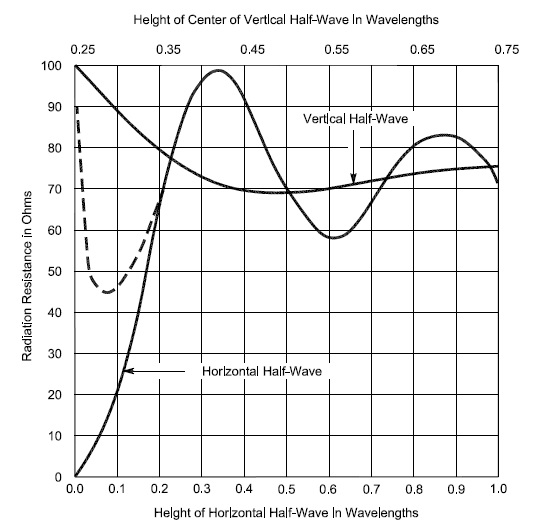 Figure 1. Radiation Resistance of a Dipole Above a Perfectly Conducting Plane. Radiation resistance values for horizontal and vertical dipoles are shown as a function of wavelength above a perfectly conducting plane. The dotted line shows how the radiation resistance of a horizontal dipole departs from the graph when the dipole is close to real ground. It is expected that the end resistance of our EFHW antenna will follow similar variations as a function of wavelength above ground, although at very different impedance levels.
This article will present test results measured at 5 frequencies in 5 bands to demonstrate how end resistances vary at a fixed height above terrain. We allow the number of wavelengths above ground to vary as a function of frequency while holding the antenna height constant. There is not enough test data to draw any conclusions other than to say that the end resistance appears to vary as a function of wavelength above the terrain. It is hoped that the measurement program will be completed as future work.
Second, if the antenna is fed close to where the radio operator will sit, as may be the case for portable operation, the electromagnetic fields at the end of the antenna may rapidly exceed those recommended by the FCC for controlled and uncontrolled environments. For this reason, it is recommended that both ends of the antenna be elevated, with the possible exception of QRP operation.
Third, any end-fed half-wave antenna will require a counterpoise. Sometimes, the counterpoise is provided by the coax that feeds the L-matching network, in which case the feedline will definitely carry common mode currents that will tend to spoil the antenna pattern of the half-wave wire. Since the coax that feeds the L-matching network steals current from the half-wave wire, it reduces the main-beam efficiency. This problem can be remedied by placing a common mode choke in the feedline at a distance of 0.05 wavelength [4] from the L-matching network. Since the common mode currents are on the outside of the shield, the value of 0.05 wavelength is measured in air, not in coax. Any effect due to the outer jacketing will be small. Be advised, however, that the 0.05 wavelength value is not cast in concrete. It is a starting point. To be absolutely sure, the currents on the transmission line shield, counterpoise, and antenna wire should be measured with an RF current probe. One such probe is the MFJ-854 [5]. As will be shown by electromagnetic analysis with EZNEC in another article, there will always be some RF currents where we don’t want them to be.
While a portion of the coaxial feedline may serve as a counterpoise, the alternative is to co-locate the common mode choke with the L-matching network so that a separate counterpoise wire can be connected to the L-matching network ground. In any event, the counterpoise conductor should be perpendicular to the half-wave radiator, regardless of whether it is horizontal or vertical, to minimize the interaction of counterpoise fields with the main antenna beam.
Methodology
A lowpass L-matching topology is employed as shown in Figure 2 – a series inductor followed by a shunt, open-ended coaxial capacitor consisting of RG-316/U. (RG-316/U coax has a capacitance of 29 pf/ft.) It is widely known that if the shunt-matching element is in parallel with the load, the transformation will be from a higher load impedance to a lower source impedance [6]. This configuration is very easy to tune. However, this configuration will not bleed static charge from the antenna wire. While a series capacitor followed by a shunt inductor in parallel with the load will provide a similar transformation and static protection, this topology is more expensive to realize and more difficult to tune. We bring this point to your attention because static protection is often omitted from antenna installations.
The matching schematic below, and tutorial from Professor Stephen Long, Emeritus, ECE, UCSB, may be found online [7].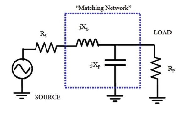 Figure 2. Lowpass Topology. The inductor may be air-wound or toroidally-wound, while the capacitor consists of an open-ended piece of RG-316/U. While the capacitor appears to be grounded at the bottom of the capacitor, for this implementation, the ground connection is soldered to the shield-end closest to the inductor. Rs is the 50-ohm source impedance, real, while Rp is the antenna end impedance, real.
An online calculator that performs all of the calculations for a variety of L-Matching Network topologies may be found on John Wetherell’s website [8]. While online calculators are great, the reader is encouraged to perform at least one calculation if only to verify that the calculator yields the same result as theirs.
A quick way to arrive at the values for the matching elements is to estimate the impedance transformation ratio required. For example, if we needed to transform from a 50-ohm source to a 4800-ohm load impedance, the impedance transformation ratio would be 1:96. From that, we obtain the unloaded Q and the reactance values required.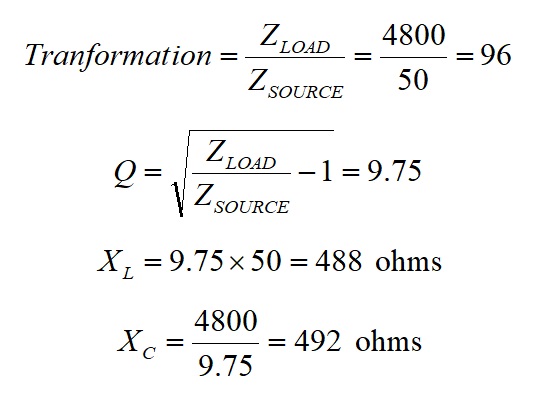 The unloaded Q = 9.75, and the reactance required for the inductor at the design frequency would be 488 ohms. The reactance required for the capacitor would be 492 ohms. If we were designing for 80m, we would calculate the inductance and capacitance from the reactance formulas at, for example, 3.6 MHz.
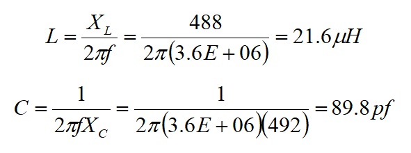 The series inductance would be 21.6 μH, and the shunt capacitance would be 89.8 pf. Then, we would build the network with a coaxial capacitor that had been cut too long and load the network with a 4800-ohm non-inductive resistor. An antenna analyzer would be connected to the network as the source, and the coaxial capacitor would be pruned a tiny bit at a time (it is easy to overshoot the mark) until the reactance at the design frequency had been canceled. If the antenna analyzer could be connected to a PC, tuning might be performed in real-time. A convenient display to use would be the Smith Chart view.
Two tables of component values at frequencies in commonly used ham bands are provided in Table 1 for CW and Table 2 for SSB. The tables are parametric and provide component values for a variety of EFHW antenna end resistances from 2000 to 4800 ohms.
A good starting value for any design is 3200 ohms, and in most cases, it will deliver satisfactory results. One need not rely upon the design frequencies in the tables. You now have all tools that you need to design networks for any frequency and any load impedance! Table 1. CW Band Segment Component Values as a Function of End-Fed Half-Wave Antenna End Resistance.
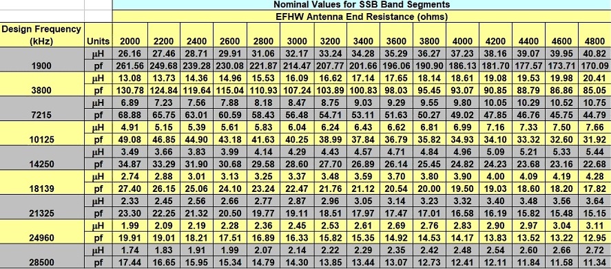 Table 2. SSB Band Segment Component Values as a Function of End-Fed Half-Wave Antenna End Resistance.
Determining Component Values
Access to an Inductance-Capacitance-Resistance (LCR) meter is highly desirable to ensure that the L-matching networks are being built to the design values. Fortunately, these instruments have become inexpensive and accurate, and they are quite useful for identifying unknown component values.
Implementation
A 30m L-matching network test article that employs an air-wound inductor is depicted in Figure 3. The sketch in Figure 4 shows the network interconnects in greater detail. The final iterated load impedance was 3024 ohms, the inductance value was 6.16 μH, and the final capacitance value was 41.7 pf. The resulting VSWR was 1.04:1 at 10.133 MHz. The air inductor was been wound on a scrap length of ½” PVC conduit. The OD of this conduit is 0.840” (21.34mm). The inductance wound for this test article consists of 22 tightly-wound turns of #20 AWG enameled magnet wire, but #18 AWG is highly recommended for the final L-matching network. Hot glue was used to hold the turns together during tests, but non-corrosive silicone is recommended once the inductance has been finalized. You can use an online calculator to estimate the number of turns required for the air-wound inductor of a specific diameter and length [9], but please use an LCR meter for precision. The capacitor consists of an open-ended piece of RG-316/U coax that was chosen for its maximum voltage rating of 1,200 volts and 29 pf/foot capacitance. The approximate length of our coaxial capacitor is 17 inches. In a separate article, we will discuss voltage requirements for transmission lines when subjected to elevated VSWR.
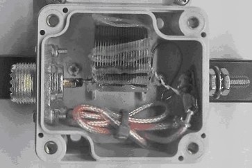 Figure 3. Lowpass L-Matching Network Topology for 30m Test Article. The air-wound inductor consisting of #20 AWG enameled magnet wire is connected from the center conductor of the SO-239 UHF connector straight through to the antenna terminal. Hot glue holds the turns in place. The coaxial capacitor center conductor is connected directly to the antenna terminal. The other end of the coaxial capacitor remains open-circuited. The photo shows a short piece of clear shrink tubing that protects the open end of the coax (see text). A ground connection to the coaxial capacitor shield is soldered near the antenna terminal end of the coax with a piece of buss wire (see Figure 3). The other end of the bus wire is grounded to the flange of the SO-239 UHF connector with a solder lug. The housing is a Bud Industries PN-1320.
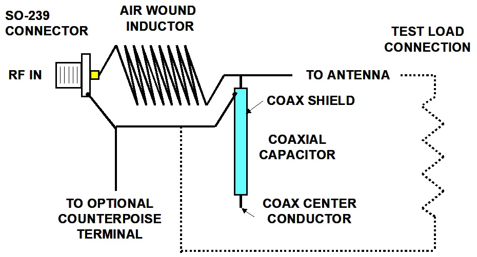
Figure 4. Lowpass L-Matching Network with Air-Wound Inductor Interconnects. The sketch shows where an optional, separate counterpoise may be connected if the coax is not used as the counterpoise. It also shows where the ground connection is soldered onto the coaxial capacitor shield. The dotted lines show where to connect the test load resistor to the network.
Figure 5 shows the configuration for a 15m L-matching network test article. The magnet wire gauge used is #18 AWG because the inductor will fit the housing. Hot glue is used to keep the turns in place. The final inductance value is 2.91 μH, and the coaxial capacitor value is 20.7 pf. The test frequency is 21.09 MHz, while the end resistance is 3042 ohms. The uninsulated open circuited coax is visible. The braid and jacket must be pruned back and insulated to prevent RF arcing. A 1 pf capacitor is soldered in parallel with a coaxial capacitor to correct the capacitance. This capacitor combination was replaced with a longer piece of coax for the final configuration.
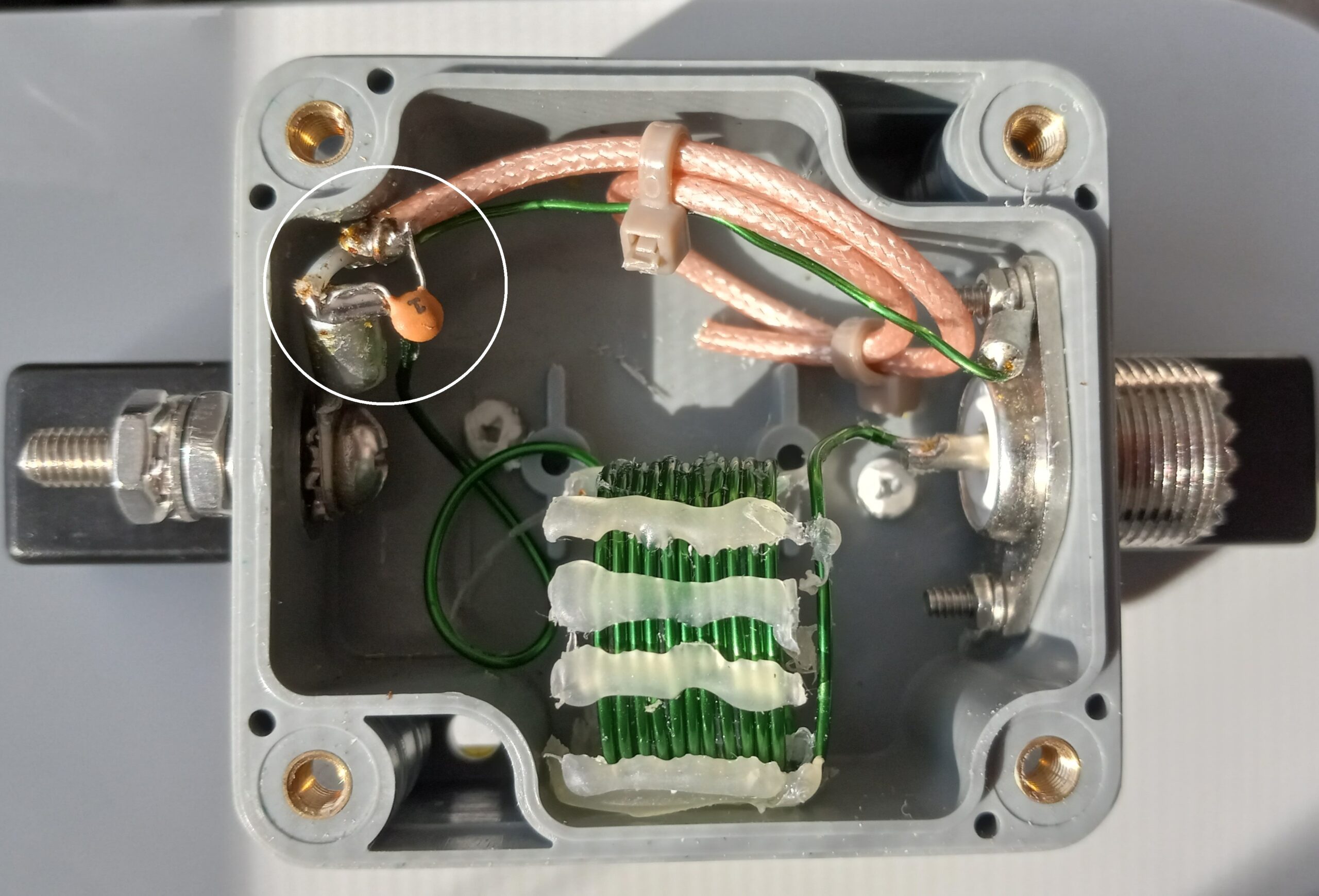
Figure 5. A 15m L-Matching Network Test Article. A 1 pf capacitor (visible in the white circle) is soldered in parallel with the coaxial capacitor to tune the network without changing the coax. The coaxial capacitor will have to be changed before transmitting because the capacitor is not rated for high RF voltage.
In order to prevent the coaxial capacitor from arcing from its center conductor to the shield near its open end, it is a good idea to snip back the coax shield a tiny bit near the open end. This has to be done while the coaxial capacitor is being tuned to its final value, however. Once one arrives at the final value, the end of the coax may be covered with a short length of shrink tubing to protect it. When tuning these networks for the higher bands, namely 20, 17, 12, and 10 meters, it may be beneficial to complete the tuning with the coax coiled in its final configuration. The pruning procedure can be somewhat fussy, and altering the capacitor configuration at the very end can lead to disappointing results.
From the network configuration, one can see that there is always access to the inductor and capacitor for measurement. It is a good idea to record the as-built values of the network once it has been tuned into the test load. Many times it will be found that the as-built values will not be exactly the same as the design values. The reason is usually the inter-turn capacitance of the air-wound coil. It’s alright as long as there is a good match into the test load resistor. We will explore the inter-turn capacitance in a separate article.
One final note on construction: The inductors for the 160, 80, 60, and 40m bands will require a large number of turns. If air-wound, they may be too long to fit within your enclosure. One solution has been to build the network in a bigger enclosure. That will preserve the low-loss properties of the L-matching network. There will be a separate article that describes the construction of a 600W L-matching network with an air inductor for 40m. For portable use, however, compactness may be a virtue, and you may wish to wind the inductors in some other way at the expense of some RF efficiency. For such cases, consider the use of small ferrite or iron cores. You will want to choose a core type for the frequency range of interest, most likely #2 (red) iron material [10] or #61 ferrite material [11]. The permeability of iron is much lower than it is for ferrite. More turns will be required on an iron core. You may also want to choose a core size that is large enough for several turns. If the core doesn’t have enough turns, it will be difficult to fine-tune the inductance. If there are too few turns, even a small adjustment will dramatically affect the inductance, and the required value will not be obtained. A 40m L-matching network that employs a toroidal inductor is depicted in Figure 6. The sketch in Figure 7 shows the network interconnects in greater detail. An FT114-61 ferrite core has been used for 40m. Eleven turns of #18 AWG magnet wire were required to obtain 10.4 μH. The coaxial capacitor consists of approximately 19” of RG-316/U. The inductance of the toroid may be altered by spreading and compressing the turns and/or by adding and removing turns.
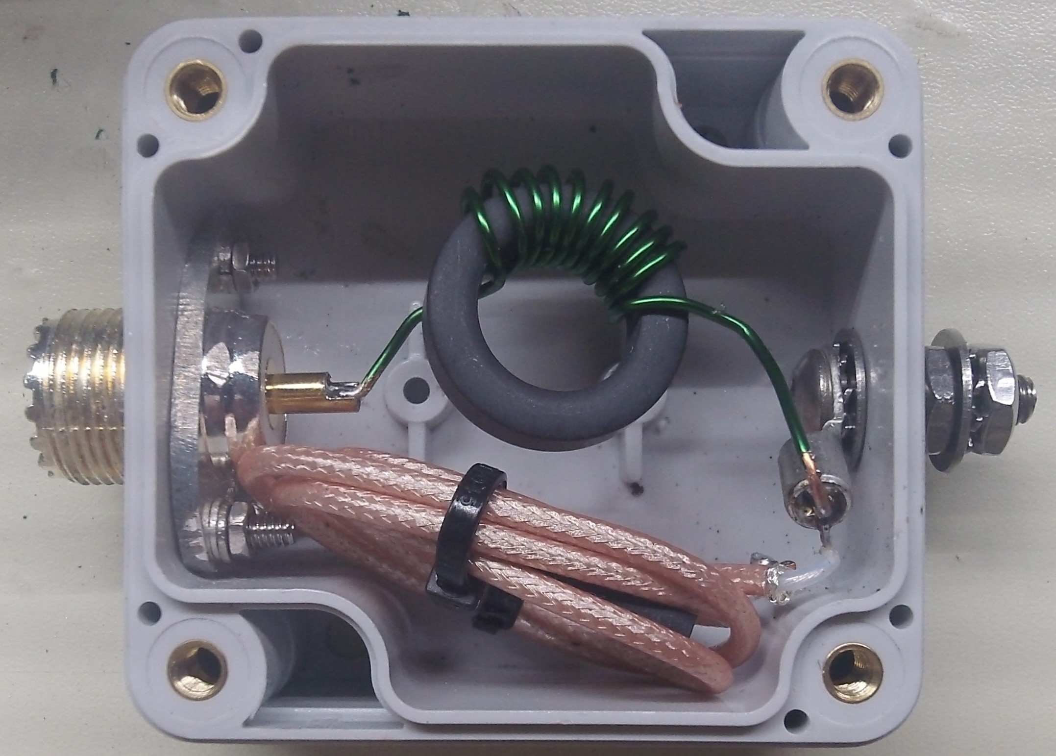
Figure 6. Lowpass L-Matching Network Topology for 40m. The toroidal inductor is connected from the center of the SO-239 UHF connector straight through to the antenna terminal. The coaxial capacitor center conductor is connected directly to the antenna terminal. The other end of the coaxial capacitor remains open-circuited. A ground connection to the coaxial capacitor shield is soldered at the antenna terminal end of the coax with a piece of buss wire (see Figure 5). The other end of the bus wire is grounded to the flange of the SO-239 UHF connector with a solder lug. The housing is a Bud Industries PN-1320.
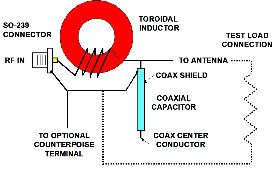
Figure 7. Lowpass L-Matching Network with Toroidal Inductor Interconnects. The sketch shows where an optional, separate counterpoise may be connected if the coax is not used as the counterpoise. It also shows where the ground connection is soldered onto the coaxial capacitor shield. The dotted lines show where to connect the test load resistor to the network.
The 80m L-matching network shown in Figure 8 was constructed with a T130-2 iron toroid core because the material was available. There are approximately 40 turns on the core for an Inductance of 21.3 μH. This core material permeability is 10, which is about one-tenth the permeability of #61 ferrite material. With so many turns, the inter-turn capacitance is apt to be large. For this design, an FT114 -61 core would be a better choice for fewer turns. This test article was built for a test frequency of 3.55 MHz with an end resistance is 4639 ohms. The coaxial capacitance value is 93.8 pf.
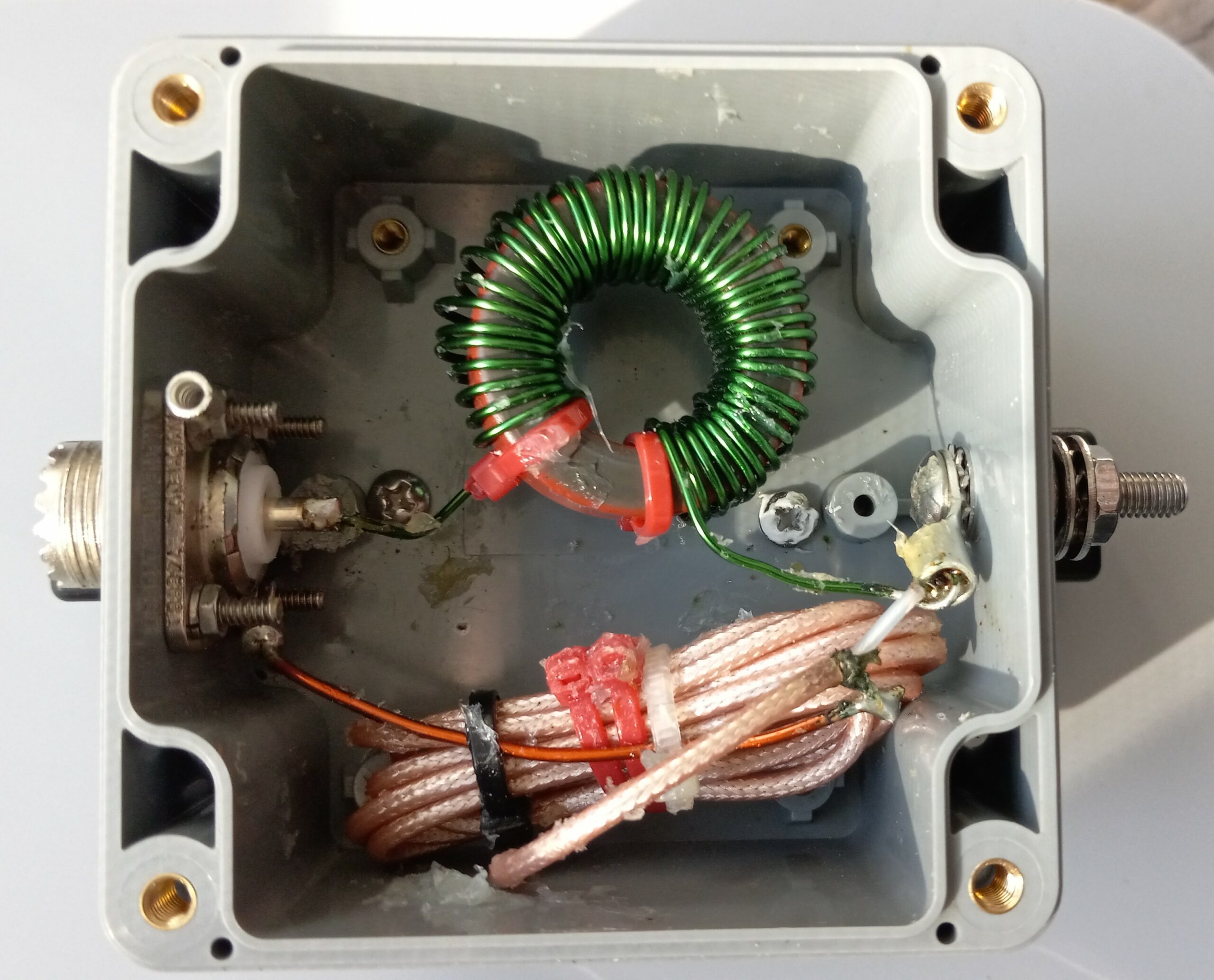
Figure 8. An 80m L-Matching Network. This network was constructed with a T130-2 iron core. The initial permeability of this core is too low, requiring too many turns with attendant inter-turn capacitance. The next iteration will employ FT114-61 material.
Lab Test Procedure
Once the design frequency and antenna load impedance have been chosen for the design, an L-matching network is fabricated. The network is loaded with a non-inductive load resistor (a cermet trimpot is a good choice), having the same value as our antenna load impedance design value. The network is connected to a vector antenna analyzer. If possible, the Smith Chart view should be utilized. Most vector antenna analyzers can be connected to a computer via USB, and a Smith Chart may be displayed in real-time. What we should see, if we sweep through the design frequency, is a display near the center of the Smith Chart. If the display is below the axis of reals for the Smith Chart, the coaxial capacitor will have to be pruned a bit at a time until the display at the design frequency is right at the center of the chart. Thus, the reactance has been canceled, and we are left with a perfect transformation from the load impedance to the characteristic impedance of 50 ohms. If we call for the reactance view on the vector antenna analyzer, we should be able to see the reactance pass through zero at the design frequency of the L-matching network. Finally, we disconnect the load resistor from the network and prepare for field testing.
A Smith Chart for the 30m L-matching network is shown in Figure 9. Data was collected on an MFJ-226 Graphical Antenna Analyzer with the network connected to a 3024-ohm cermet trimpot test load. Once the inductance had been adjusted with an LCR meter, the coaxial capacitor was pruned until the reactance was canceled to place the cursor at the center of the Smith Chart. The network was designed to match 3000 ohms, and a slight adjustment of the trimpot placed the cursor at the center of the chart. Tuning is a bit tricky because the 30m Band is so narrow.
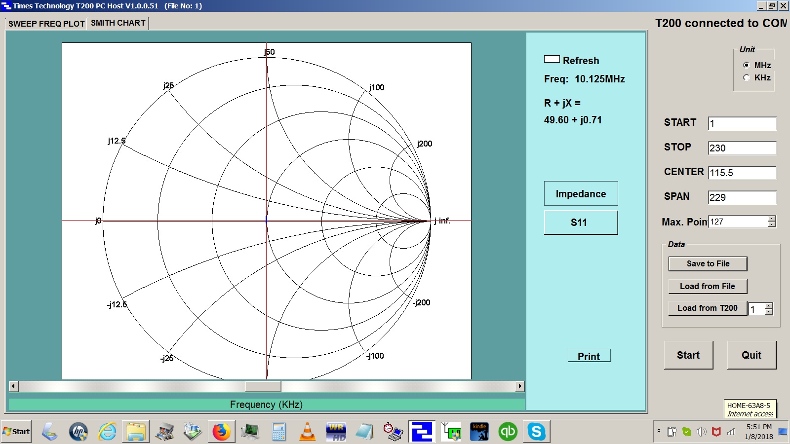 Figure 9. Lab Tuning of the 30m L-Matching Network. The inductor, capacitor, and test load are adjusted to place the cursor and the center of the Smith Chart.
The VSWR performance of the 30m L-matching network is shown in Figure 10. Excellent performance has been achieved over the entire band after lab tuning. Figure 10. VSWR Performance of the 30m L-Matching Network. Excellent performance has been achieved over the entire 30m Band.
The 40m L-matching network of Figure 6 was tested in the lab. The network was loaded by a 4573-ohm load. The resulting Smith Chart that was swept over the entire 40m band is shown in Figure 11.
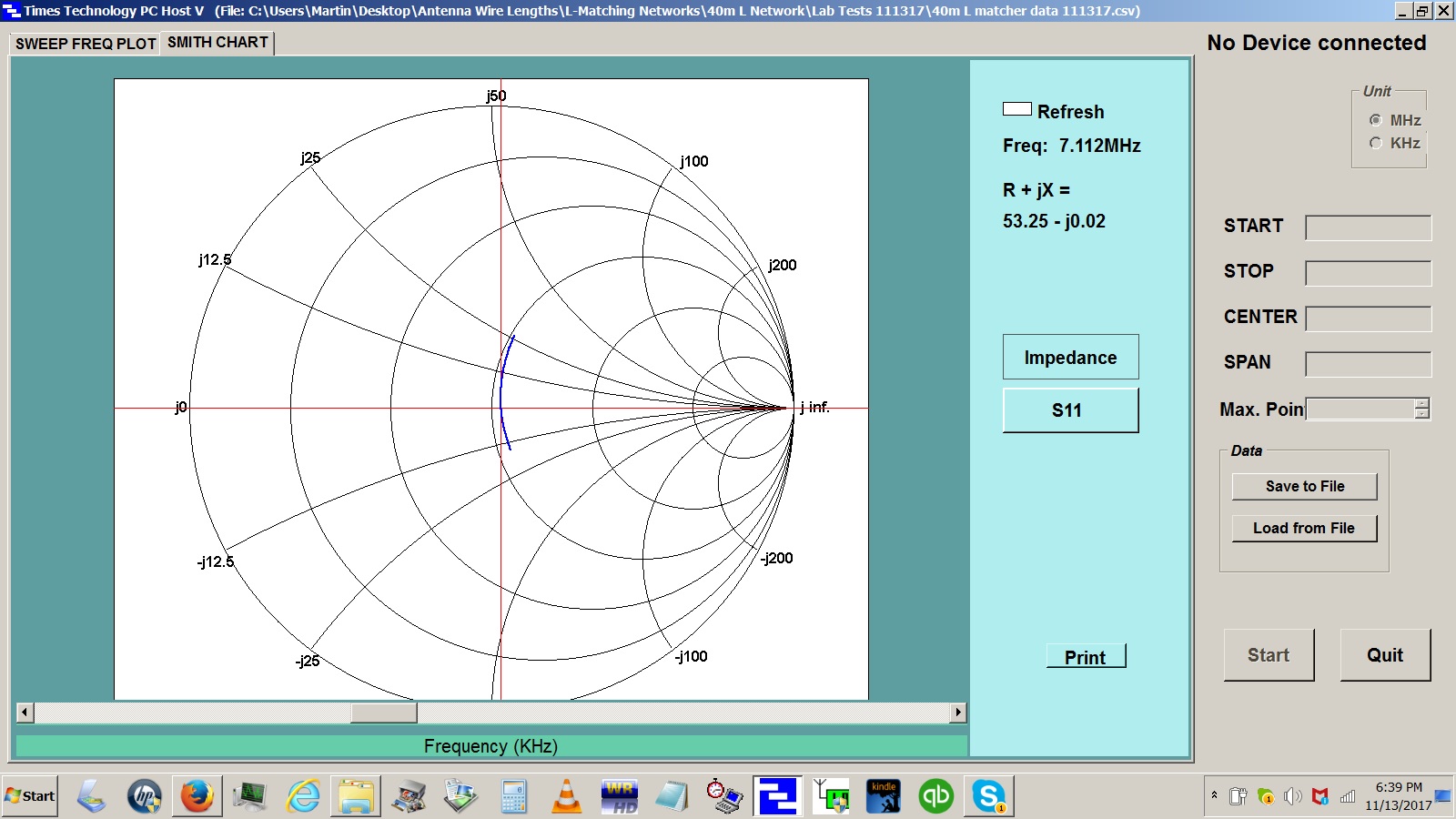 Figure 11. 40m L-Matching Network Smith Chart. An excellent match is observed over the entire band.
The VSWR performance of the 40m L-matching network is shown in Figure 12. Excellent performance has been achieved over the entire band after lab tuning.
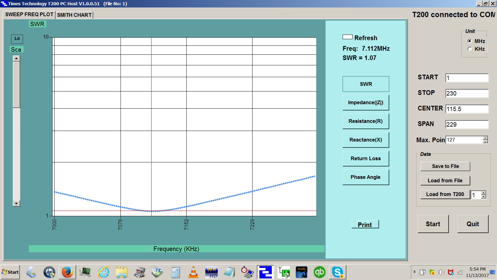 Figure 12. VSWR Performance of the 30m L-Matching Network. Excellent performance has been achieved over the entire 40m Band.
Field-Test Prep
In preparation for field-testing, we will want to prepare the counterpoise that will consist of a length of coax that has been cut to 0.05 wavelength at the design frequency. If the common mode choke will be connected to the L-matching network at the SO-239, a wire should be cut to 0.05 wavelength at the design frequency. A grounding stud should be provided to the network ground for counterpoise connection. This may be a separate ground stud mounted on the case and connected to the SO-239 connector flange, for example. Please refer to one of the interconnection diagrams for the counterpoise connection point.
Field Test Procedure
In order to test the EFHW antenna with an L-matching network feed, two end supports will be necessary. The supports may be a pair of nearby trees, a pair of telescoping masts, or one of each. Each support should be fitted with a halyard so that each end may be raised and lowered. Ideally, testing should be performed at least 0.25 wavelength above ground, except, of course, for the case of an inverted-L. The L-matching network and common mode choke will be heavy, so the end support has to be sturdy enough to support the weight of the transmission line, matching network, counterpoise, and choke. Once that is arranged, testing may begin.
Without altering the L-matching network or counterpoise in any way, the length of the antenna wire should be pruned to cancel any remaining reactance at the design frequency as viewed on the antenna analyzer. Once that has been accomplished, the real part of the impedance may be read. It should be close to 50 ohms. If it is not, then we know that we have chosen the incorrect impedance transformation ratio and, consequently, the incorrect value for unloaded Q.
Figure 13 shows the field-test Smith Chart for the 30m L-matching network. The swept measurement places the cursor very close to the center of the Smith Chart. The actual performance is very good for the entire 30m Band.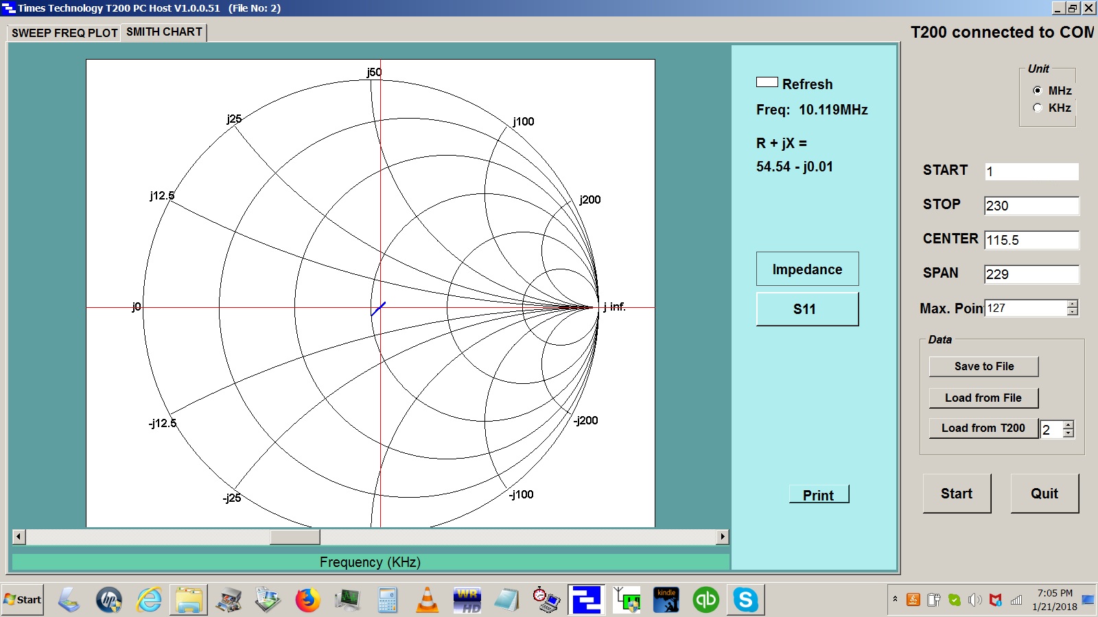 Figure 13. Field-Test Smith Chart for the 30m L-Matching Network. Measured performance is very good over the entire 30m Band.
The field-test VSWR performance of the 30m L-matching network is shown in Figure 14. Excellent performance has been achieved over the entire 30m Band.
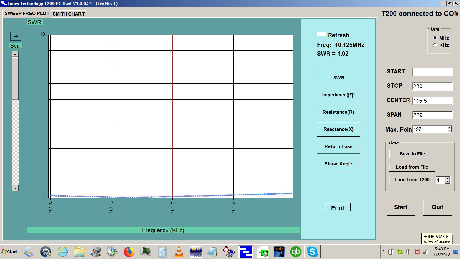
Figure 14. Field Test VSWR Chart for the 30m L-Matching Network. VSWR performance is very good over the entire 30m Band.
If the VSWR is satisfactory, testing may be completed. If it is not, iteration is the next step. Usually, the real part of the transformed antenna resistance will hint at whether we have chosen a transformation ratio that is too high or too low.
There is another approach that is worth considering. An L-matching network can be constructed from a tapped series inductor and a shunt air variable capacitor. Calculations may be performed in the field to alter the impedance transformation ratio by adjusting the inductor and capacitor. Once satisfied with the result, the inductor and capacitor values may be made permanent. If you happen to have a home with a second-story window, you might consider stringing the antenna from the window out to a tree or mast. Then, the L-matching network adjustments can be made from the open window. Please take care to keep children and pets away from any open window.
In any event, the antenna wire length will have to be restored to its full starting length so that it may be pruned enough to cancel any residual reactance that might be observed for the iterated L-matching network. Tiny wire rope cable clamps [12] shown in Figure 15 provide a way to splice pieces of wire back onto the antenna.
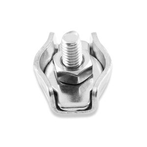 Figure 15. Wire Rope Clips. The 2mm and 3 mm variety are handy for splicing pieces of antenna wire together.
By now, you have probably figured out how to perform some reverse engineering from the field-test results. If the values of the inductance and capacitance have been determined experimentally, it is possible to work backward to determine the unloaded Q and then the impedance transformation required to obtain a match. From this, you will be able to estimate the end resistance of the wire.
Field Test Results
Some field-test results are summarized in Table 3. Many of the load impedances for the L-matching networks have been iterated, and these values appear in the table. Because of weather considerations on the test range in Florida in spring 2020, the test program was suspended. Nonetheless, all of the networks were tested and iterated, with the exception of the 80m L-matching network. This may have been fortuitous, as there was no means to elevate the 80m antenna to a height exceeding 0.25λ (66 ft) with the masts available.
All of the measurements in Table 3 were made with 50′ of RG-8X coax. The reference plane of each measurement was moved to the plane of the SO-239 connector on each L-matching network by means of an open/short/load calibration load kit.
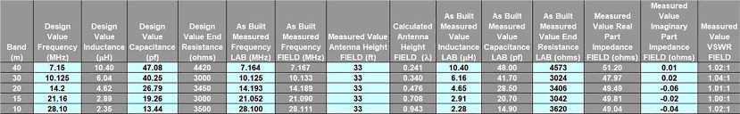 Table 3. Spring 2020 Field-Test Data Summary. The as-built component values and VSWR results are as reported. The L-matching networks and coax were supported by a 33’ (10m) mast. The mast was judged to be of insufficient strength to support an additional common mode choke. Consequently, all measurements were made with a 50’ length of RG-8X where the entire coax acted as the counterpoise. No attempt was made to optimize the length of the counterpoise. The 80m L-matching network could not be tested because of the weather. See text.
References
[1] ARRL Antenna Book, 21st ed., Ch. 7, p. 2.
[2] https://www.eznec.com/
[3] Blustine, M., L-Matching Networks – Field Measurements, March 17, 2020.
[4] https://www.aa5tb.com/efha.html
[5] https://mfjenterprises.com/products/mfj-854
[6] https://web.ece.ucsb.edu/~long/ece145a/Notes5_Matching_networks.pdf
[7] Ibid.
[8] https://home.sandiego.edu/~ekim/e194rfs01/jwmatcher/matcher2.html
[9] https://www.66pacific.com/calculators/coil-inductance-calculator.aspx
[10] http://www.qrz.lt/ly1gp/amidon.html
[11] https://www.66pacific.com/calculators/toroid-coil-winding-calculator.aspx
[12] https://www.amazon.com/Rannb-Stainless-Simplex-Single-Diameter/dp/B07DLVNR54/ref=sr_1_7?crid=26694JFBAHN04&keywords=cable+clamp+3mm&qid=1654922072&sprefix=cable+clamp+3mm%2Caps%2C85&sr=8-7
Martin, K1FQL
Lagarde Capitulates As the Euro-Zone Divides by Tom Luongo
I know you probably get tired of me saying this but the Euro-zone is headed for a massive crisis. On Thursday, June 9th, the ECB came out with its policy statement, less than one week before the next FOMC meeting statement (June 14th).
It was a doozy. Christine Lagarde attempted early on to project that soothing calm central bankers are supposed to exude even when everything is collapsing around them.
But, truly this was Lagarde’s ‘Baghdad Bob’ moment. She stood up there and read the ECB’s policy statement off the teleprompter like she had something caught in her throat, likely the remnants of what is left of her conscience, because even she couldn’t swallow the bullshit she was slinging.
We have inflation under control. We will still grow in 2022 (BWAHAHAHA!) and growth will accelerate in 2023 and 2024. These people haven’t gotten one quarterly forecast right in … forever, and yet they project this idea that they have any clue what GDP growth will be in 2024?
But, as Zerohedge pointed out, Lagarde then reversed herself during the press conference, trying to resurrect the ghost of Mario Draghi, saying that she stands ready to do ‘whatever it takes’ to stabilize the situation.
From ZH:
She notes there are existing instruments with the reinvestment capacity under the PEPP.
“And if it is necessary, as we have amply demonstrated in the past, we will deploy either existing or new instruments that will be made available.”
Lagarde states that “within our mandate we are committed to preventing fragmentation risks within the euro area.”
So some kind of asset purchase scheme for peripherals? The vagueness is intentional as it appears Lagarde is trying to pull off a Draghi ‘Whatever it takes’ moment while keeping her foot on the hawkish pedal.
As The IIF’s Robin Brooks pointed out:
If the ECB says to markets: “we will defend Italy’s spread,” markets will for sure test that statement. So – in effect – what the ECB did today is to raise the odds of markets trying to force its hand.All this is avoidable. Don’t hike. The Euro zone is going into recession…
The end result was obvious to anyone with ears to hear, we are reluctantly following the Fed’s lead in ending QE hoping that someone will still think that Italian BTP’s trading at 65 bps above US Treasuries of the same maturity is a ‘good deal,’ and invest in a country that now carries increasing redenomination risk.
If it wasn’t so over-the-top moronic, it would be funny. Now with the horrific US CPI print red-pilling a whole lot of investors that the Fed has the green light to be even more hawkish, the mad scramble is on to figure out where to park that money that’s been frozen by the clown show that is US domestic politics.
The Fed’s in control here, but not in the way a lot of people think. The next level of insight that should begin to take hold, especially if the next CPI print is equally awful, will be what I’ve been saying for a year now….
The Fed isn’t raising rates to combat inflation. The Fed is raising rates to break the ECB and Davos.
Spread Eagled ECB
Two months ago Italian debt, thanks to Lagarde’s lying and everyone’s front-running her trades, was trading at a premium to US debt. Um, Chrissy, you’re going to need to see that spread vs. US debt be more like 650 bps (6.5%) rather than 65, if you want to attract even the average NFT investor at this point.

The bond markets are all now moving away from the monetary experiments Lagarde inherited from Mario Draghi and she has neither the experience nor the gravitas to carry this charade off any longer.
The big takeaway, and the reason why the euro had a mild bout of myocarditis thursday morning before collapsing on its way to the bathroom, is because Lagarde is open to creating a new, improved, QQEternity, alphabet soup program in the future if this ending QE ‘experiment’ doesn’t work.
With the Fed now secure in its role as European liquidation agent, there’s nothing Lagarde can do other than follow the yellow brick road to make the best of a terrible situation getting worse by the day.
That said, I have to ask the serious question, are they really worried about Italy at this point? It’s not like the folks at Davos Central didn’t manipulate the Italian political scene to achieve exactly this state of affairs. So, I honestly don’t think they care at all about Italy.
In fact, I’d argue that they would rather have Mario Draghi ride Italy into the ground and turn the country into a smoking ruin in the hopes of saving the northern European currency bloc.
The whole point of putting Draghi in charge was to liquidate Italy. Italy’s financial implosion would be just the cause celibre Davos has been trying to create to consolidate power within the ECB by taking complete control over its banking system when all the banks collapse.
Think back to the Banco Popular implosion where it was forcibly liquidated by Draghi when he was ECB president and sold to Santander for $1. The power that Draghi exhibited there was astounding. And it was a warning shot to investors that no one’s money is safe from the commissars at the ECB.
While Draghi kept things together through strong-arming and, at the times, a sympathetic FOMC with Janet Yellen at the helm, the precedent was set then that the ECB has power over its member banks that the Fed doesn’t have. Today, looking at the situation, I’d say this is a very good thing.
You’re going to see a lot of this going forward in Europe and too many commentators are not prepared for the idea that this is all deliberate.
It’s not the plan they wanted, which was for this collapse of the Euro-zone to occur on their timetable not the markets, but it’s still the plan. They hoped they’d have a compliant Fed putting the New York banks on notice that they have no friends left.
Davos may be improvising here, because the Fed is clearly working them over the coals as Eurodollar markets dry up, but they are still trying to make the best of a bad situation.

And that’s why Lagarde was trying to soften the market up by saying, “We have everything under control and still have tools.” It’s all you ever hear from these central bankers, when, in reality, they have zero real clue anymore than we do.
If the European banking system collapses in the way I am forecasting this is what will destroy the Eurodollar markets, as those banks which previously levered up their dollar balances will have zero ability to do so after they are absorbed by the ECB.
Once this potential outcome is truly digested by the markets, and I think Friday’s complete shitshow was the beginning of that realization, then that’s when we are going to see rapid shifts in bond spreads, O/N money market rates and blow-outs in things like 1 month and 3 month USD LIBOR.
Speaking of that, the SOFR/1month LIBOR spread blew out to 44 bps on Wednesday. After the ECB’s performance and the worse than expected US CPI print (8.6% vs. 8.3% expected), I’m having a hard time believing we won’t see a wider spread than the 53 bps we saw the day of the last FOMC meeting by Wednesday’s next FOMC meeting.

The Political Fallout
What is most important here is that the ECB being exposed as having no ‘there there’ undermines the political positions of nearly every major politician across the euro-zone. It’s not like a banking crisis is going to make Olaf Scholz’ coalition in Germany stronger or Draghi’s caretaker government in Italy.
These guys will finally begin to feel real political anger for change as inflation eats away the middle class, high energy prices gut corporate profits and there is no end to the regulatory tyranny coming from Brussels, hell bent on forcing an anti-hydrocarbon agenda down everyone’s throat.
That said, you know Davos will try to keep a tight lid on the EU’s core, because it carries the most political power. What they won’t be able to control, once this begins to unravel, is what the so-called periphery does.
Bulgaria’s Davos-backed government lost a key partner recently. Boris Johnson is toast in the UK as the Night of the Tories Long Knives has come and gone. No one knows how to turn on their leadership like the Tories — Thatcher, May, now Johnson.
Turkey has all but declared war on Greece over Erdogan’s creative interpretation Greece’s sovereignty, accusing it of militarizing islands in the Aegean. Estonia lost its majority over inflation not caused by Russia, but by their own rabid Russophobia.
The economic realities of what Lagarde et.al. have set in motion but can’t control will be the collapse of nearly every major government in Europe over the next year or two while incentivizing countries like Hungary to declare independence from Brussels.
This is why Lagarde was so keen to remind us that she is aware of ‘fragmentation risks’ and that she’s on top of it. Too bad this is more bucking bronco than bucolic burro. I’ve got the under on whether she lasts the 8 seconds or not.
The key is Russia continuing to grind out victories in Eastern Ukraine while using the time to reinforce its positions in the south and expose the utter bankruptcy of the West. I told you that this was a race to someone’s Great Reset, not necessarily Davos’ when the war broke out.
Putin is upping the operational tempo on the neolibs of The Davos Crowd in Europe and the White House as well as their neocon useful idiots in the US/UK foreign policy circles, Congress and intelligence services to create the ultimate geopolitical Russian cauldron for their avarice.
Ukraine represents everyone’s existential threat.
If the neocons lose, they are done as an influence within foreign policy circles in the West forever because they will have failed to penetrate Fortress Russia.
If Davos loses, their grand plans for global domination become diminished to, at best, the European Union and some parts of the Commonwealth.
If Russia loses, the entire Global South, fails to escape the fiat, debt-based slavery of the Western central banking cartel, because they will control the flow of Russian natural resources in such a way that they will not be stopped. More on this later.
After Bojo the Bozo in the UK the big question is who’s next?
There’s a lot of speculation that the German government will fall, but I’ve seen this story play out in Italy before. The coalition could fail and the President Frank-Walter Steinmeyer, a Davos man through and through, will refuse to sanction new elections and should force the parties to cobble together a new technocratic government that will be indistinguishable in policy from the existing one.
Since the Greens are embedded in nearly every state delegations to the German Bundesrat (upper house) there will be no real policy change since they control what legislation actually gets passed.
This is why Scholz is so weak.
Since each state in the Bundesrat votes as a bloc, the Greens control 41 of the 69 votes there, giving them effective control over policy. This was Merkel’s greatest achievement while Chancellor while also bamboozling Putin in to thinking the Minsk agreements were something other than a time-waster while NATO built and trained the Ukrainian army his men are now pummeling into dust.
This is what she set up with each of the state governments, by refusing any AFD coalitions to form in any state, she ensured that no matter what happened, there would be no challenge to the Greens revolution of Germany’s legislative agenda.
Davos is setting up the failure of the German government to hand it to Brussels. So, if the German government fails and Steinmeyer refuses to go for new elections, then the resultant caretaker government will be even weaker than Scholz’ government and ensure the complete betrayal of the German people to the EU.
And the worst part will be that they will still feel like they have control over what happens to them next because the German people are still told they control EU policy at the top.
When in reality all that will happen is the EU will fracture along capital efficiency lines and the euro will drive it into bankruptcy, forcing real political fracturing. Eastern Europe will break off the moment the EU tries to enforce the energy embargo on Russia, especially if Russia gains Odessa and access to the Danube river system. Watch Bulgaria carefully as the next Soros-backed junta to fall completely to the economic reality of a dying EU.
Good job, Chrissie, you’ve achieved the exact opposite of what you intended, which is a unitarian banking and political system. Because, as always, people respond to incentives. In the US, we said no to Climate Change, CBDC’s and gun control. In Russia, they said no to debt and Nazis. And in China, they simply said no to oligarchs who weren’t Chinese.
Pretty easy to tear up the EUSSR under this scenario. Pretty easy to see what happens next.
Subscribe to:
Posts (Atom)