Montana Motor Stables: A Versatile Tuner for SOTA Activations by George KX0R

Monday, October 28, 2019

A Versatile Tuner for SOTA Activations by George KX0R

Numerous tuner designs are available, and endless possibilities exist for combining tuners and antennas to use for SOTA. My tuners have evolved through experimentation and modification. I want to share my current tuner design, so other SOTA activators may enjoy the benefits of similar tuners. I’ve had consistently good results using these tuners. This is intended to be a manual to share what I have learned.

This is a detailed, technical piece, intended mostly for “makers” and more creative activators, who enjoy building and using their own tools on the summits. My drawings are crude, but the content is powerful.

We recognize these key points:

Most portable radios require an impedance near 50 ohms at the antenna port.
Most real antennas don’t present an impedance of 50 ohms at frequencies we use
A tuner is a device to change the impedance of our antenna to about 50 ohms
A tuner performs complex functions to transform the antenna’s impedance
We don’t need to understand the mathematics of impedance matching to use a tuner
We do need to understand the basic concepts of what a tuner does to use it effectively
Mathematical theory, involving complex variables, is required to understand impedance-matching devices
Tuners can be modeled with available software
Some key intuitive concepts can take us far enough that we can make successful tuners
Bench experiments and field tests can yield acceptable results
An antenna does not have to be resonant in order to radiate effectively at various frequencies

The impedance of any antenna can be expressed as two variables: resistance R and reactance X.

Z = R + jX

Z is a complex number, with j = SQRT of -1.

In order to change the actual Z of the antenna to a simple resistance of 50 ohms, our tuner must do two things:

Change the antenna’s actual R to 50 ohms
Supply an opposite reactance to cancel out X

To match an antenna’s complex impedance, ideally, we could do this procedure:

Measure the complex impedance with an analyzer
Design a network of L and C components to transform the impedance to 50 ohms
Build the network and test it - verify that the impedance has been transformed to 50 ohms

For our antenna to work on several frequency bands, we would analyze the antenna at various frequencies of interest, design and test matching networks, and then configure and package the matching device(s). We might decide to change the antenna as well, leading to more work.

With so many choices in the process, we might spend a lot of time and effort trying to come up with a practical antenna and impedance-matching device that would work well in the field.

Faced with this tricky puzzle, many ham operators take shortcuts in order to get on the air more quickly:

Purchase a ready-made “solution”, often an antenna with a broad-band matching network
Purchase a limited manual tuner with some attractive features
Purchase an auto-tuner
Use an antenna they think is 50 ohms - but usually isn’t!
Try some other clever tricks that others suggest

The results vary greatly, but if radio contacts happen, many operators continue to use their compromised equipment, unaware of what they’re missing.

A different approach is presented here:

We accept that antennas are mathematical functions, in which R and X vary with frequency
Voltage and Current are not usually in phase at the feedpoint, i.e., the load is a complex number
Voltage and Current may vary over a great range of values at the feedpoint
We don’t know what Z is, but we won’t analyze our system in detail, only very generally
We create versatile networks of components that can transform a wide range of complex impedances
We include enough variables in these networks that we can achieve a desired match in a few seconds
We include a device to indicate visually when we have a match, i.e., the feed impedance is 50 ohms resistive
We learn to use these devices in the field and make improvements over time
We accept that our tools include compromises, so we need to be aware of limitations

Impedance-matching devices consist mostly of inductors and capacitors combined in various configurations. Many popular circuits have been developed, all with various trade-offs in performance. We must decide how much complexity we can tolerate in order to get the performance we want.

My original design goals:

Multiple bands – 40-30-20-17M
50 ohm input
10W RF power
Match 25-5000 ohms resistive
Match wide range of reactance
Optimize for unbalanced loads, end-fed wires, etc.
Also use with balanced loads, dipole, loop, etc.
Minimal size – weigh a few ounces
Low cost
Durable enough for SOTA activations
Accurate visual indication of 50-ohm match
Use with counterpoise or not
Good efficiency
Use for SOTA activations in the Rocky Mountains of Colorado

NOT Goals:

Cover the entire Smith Chart
Simple and easy to use by others
Foolproof
Minimize cost
Design for production
Tune automatically
Digital or remote control, etc.

Next, I show a series of concepts progressing to a practical tuner topology. The end result is relatively complex, but it provides plenty of performance in a tiny package. Most of the lower-cost alternatives are simpler, with fewer features, but they may perform OK, if you stay within the constraints of their designs.

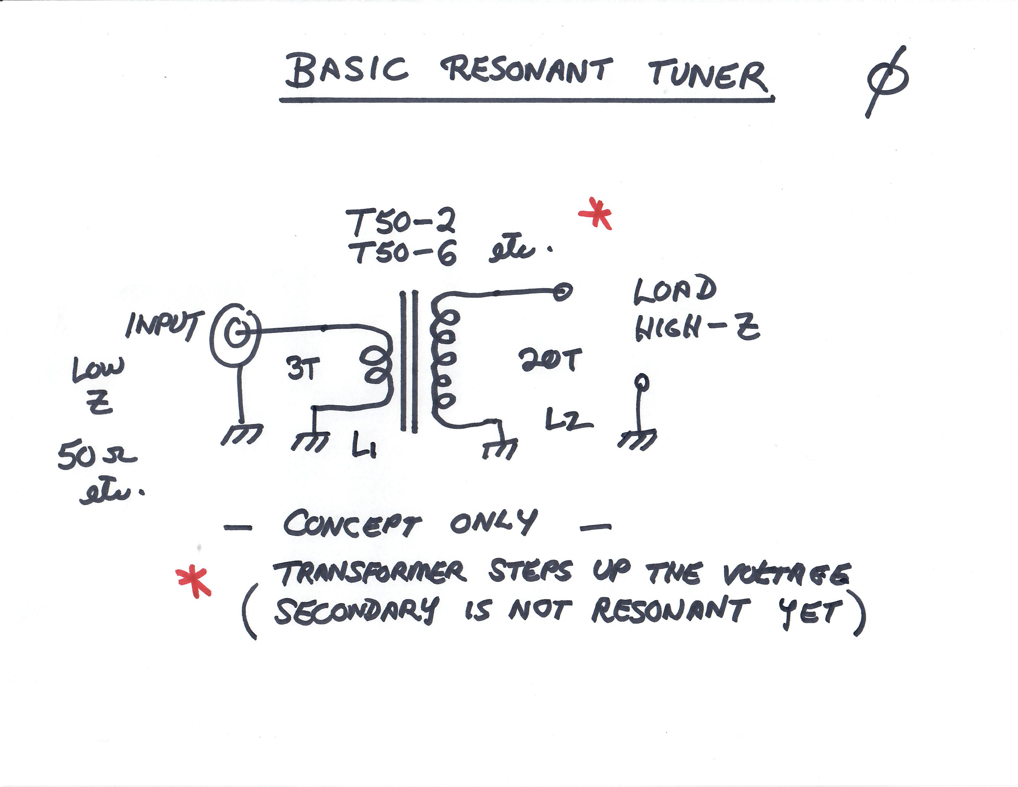
BASIC RESONANT TUNER 0

A conventional transformer is wound on a powdered-iron toroid core. This increases the impedance from 50 ohms to some higher value, depending on the turns-ratio of the windings L1 and L2. This is the basic concept of all the tuners included here.

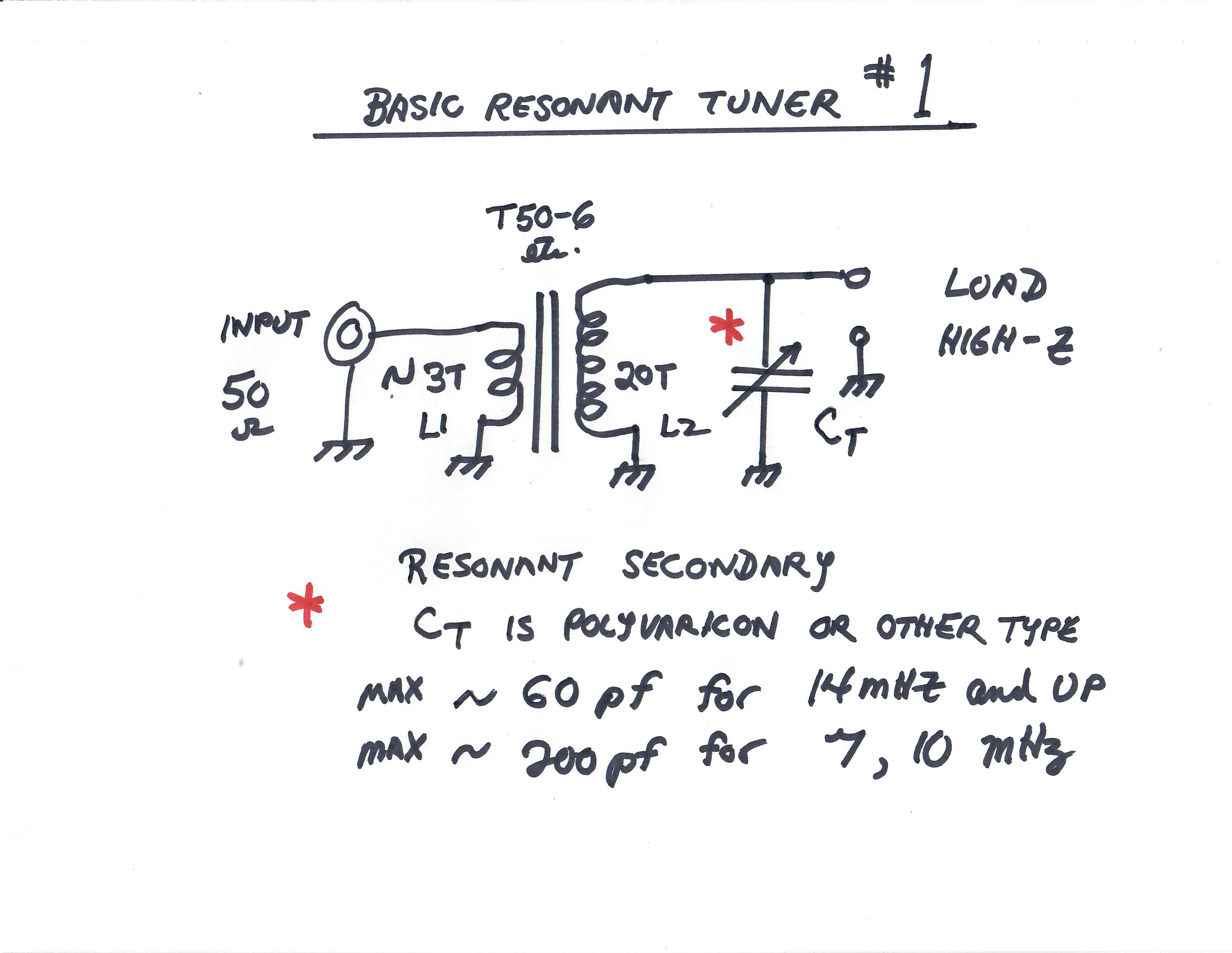
BASIC RESONANT TUNER 1

A variable capacitor across L2 is added . This allows parallel tuning the secondary, so that it can correct some reactance presented by the high-Z load. The impedance step-up can be adjusted by changing the turns ratio of the windings L1 and L2. The turns shown are just examples, concept only.

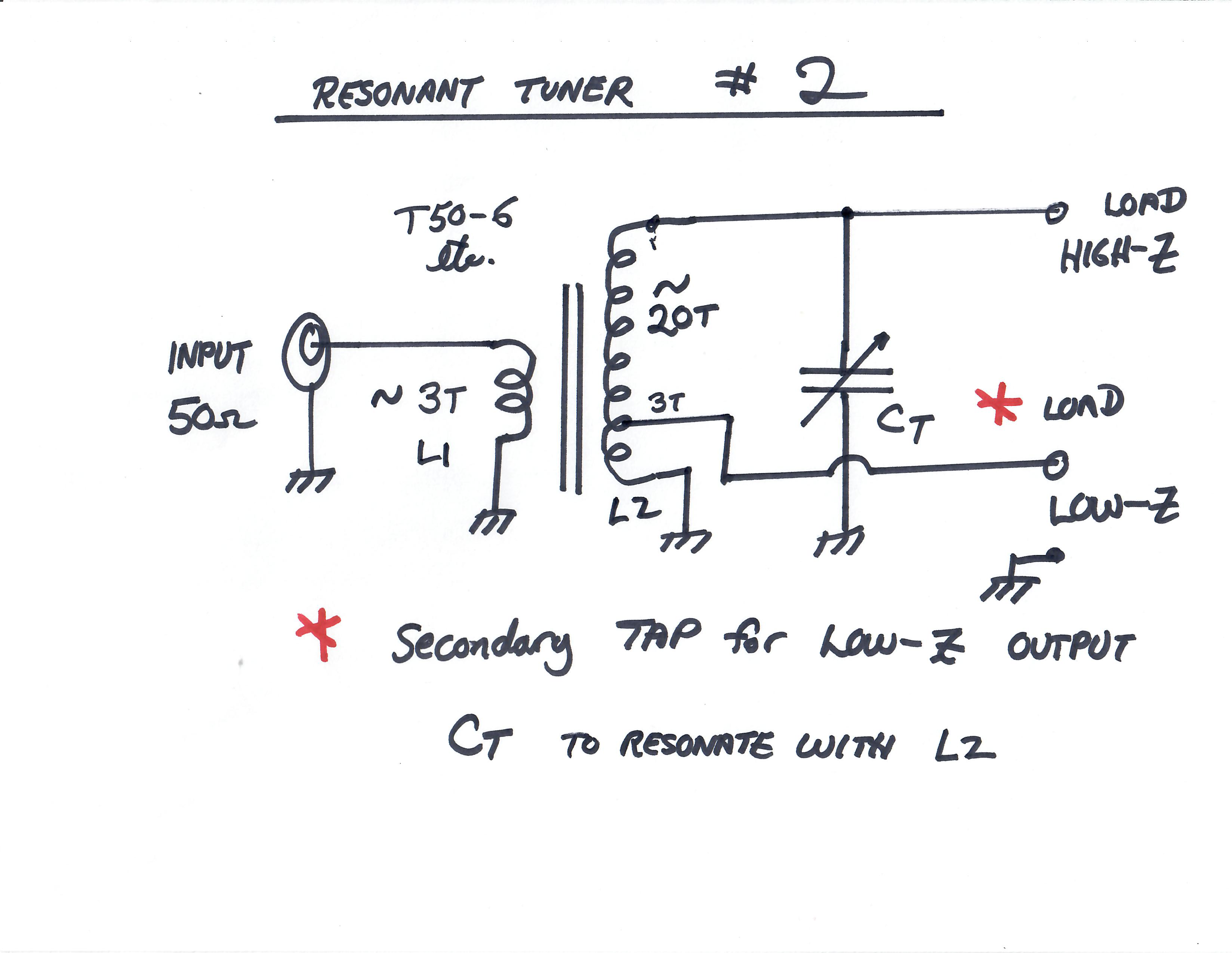
BASIC RESONANT TUNER 2

A tap is added to the secondary winding, so that a lower voltage can be selected for a second output connection. This is for a much lower-impedance load. The impedance output of the new tap is controlled by its position on the winding. Position shown is just an example.

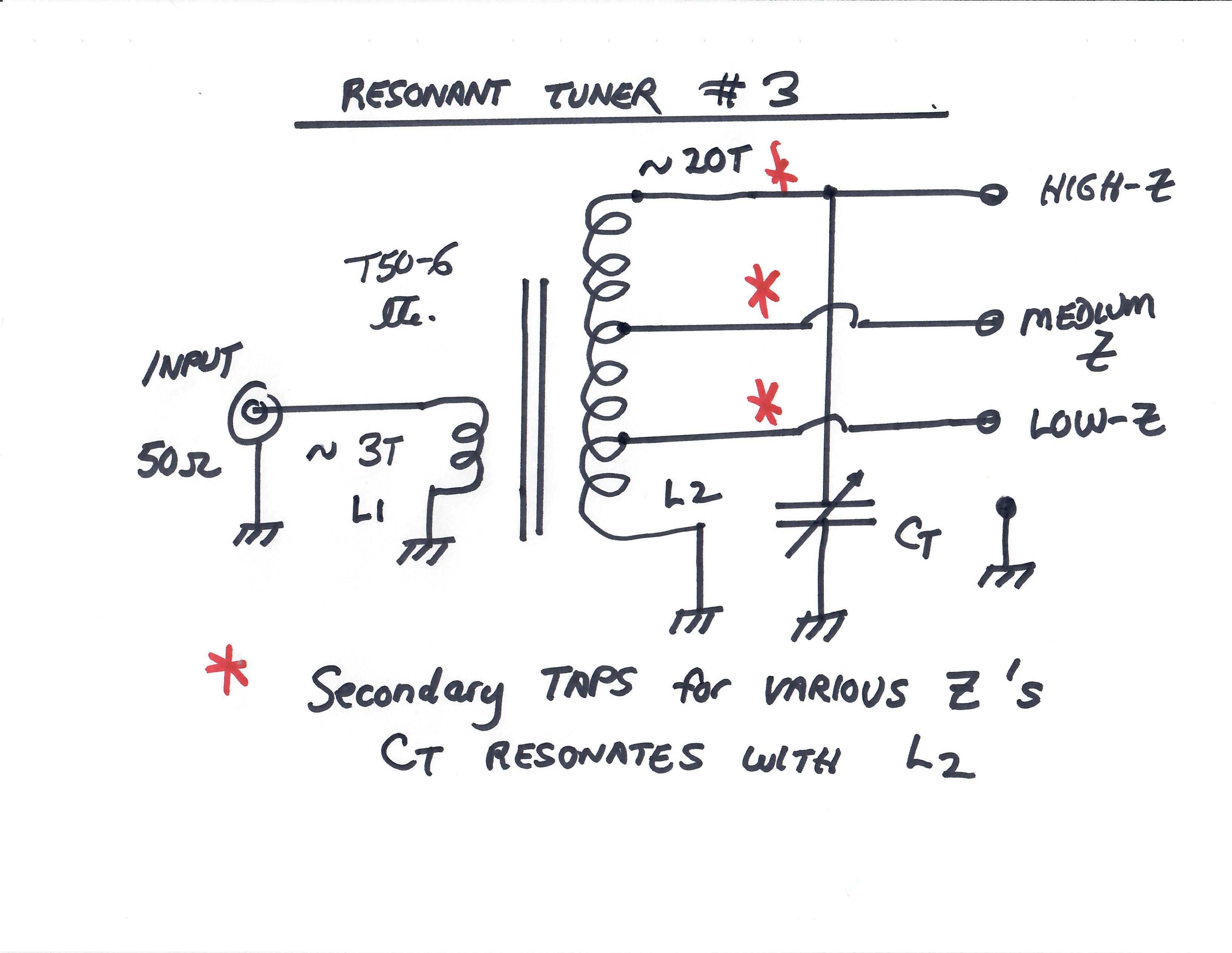
BASIC RESONANT TUNER 3
More taps are added to the secondary, so that a greater range of impedances can be matched. These outputs may be connected to separate terminals, or a rotary switch may be used to select the active tap.

BASIC RESONANT TUNER 4

In all the previous examples, we can tune the secondary to resonance with CT. We also have some control of the coupling and impedance transformation by choosing the primary and secondary turns, when we wind the transformer.

In this example, a variable capacitor is placed in series with the low-impedance primary winding. This “input capacitor” is chosen to create a series resonance with the primary winding, more or less.

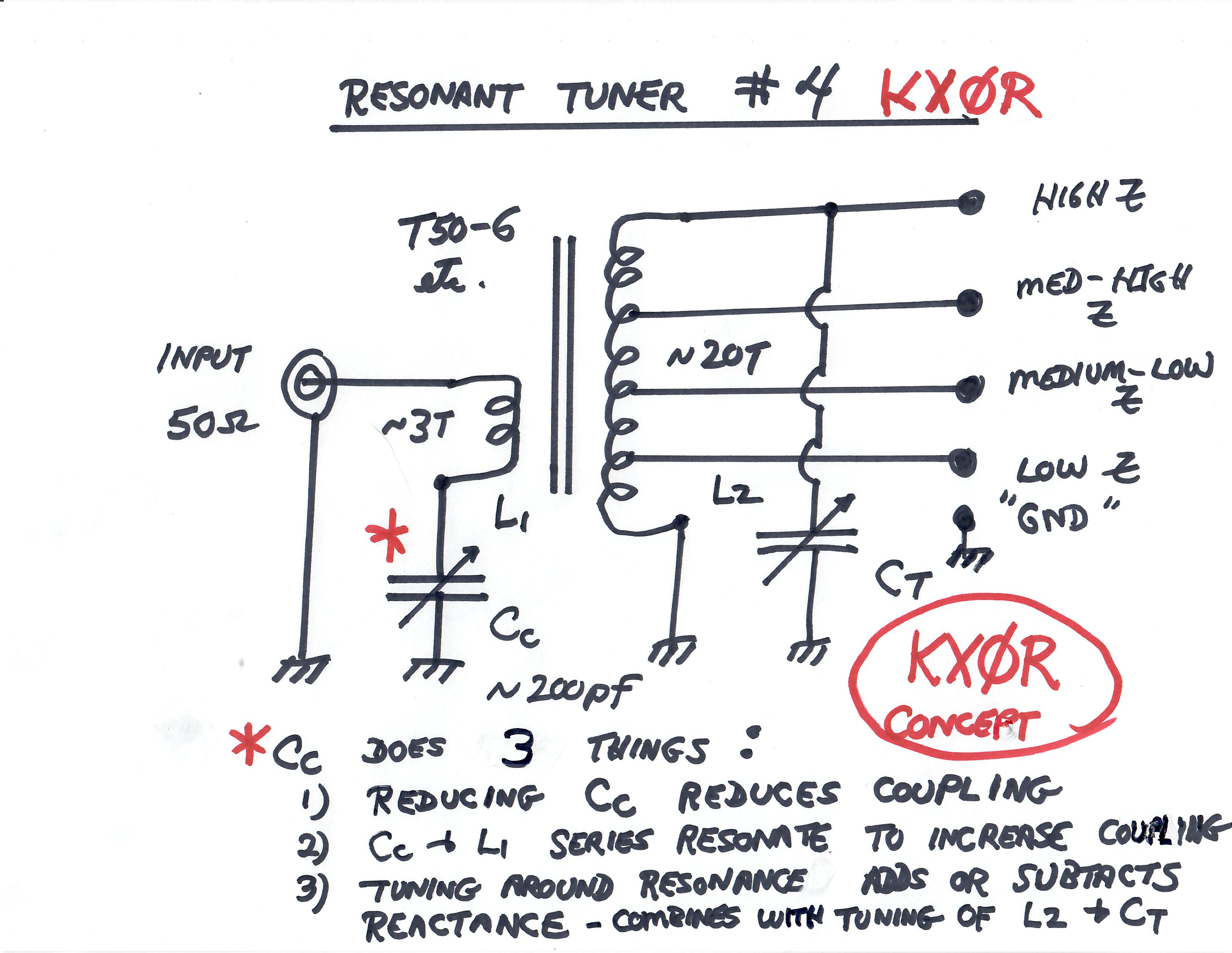
This series capacitor has a very powerful set of effects on the transformer:

When L1 and CC are tuned near series-resonance, the coupling between the windings is increased, because more current flows in the primary winding L1.
As we tune the primary circuit off-resonance, we both change the coupling and add or subtract reactance from the input network.
A new voltage transformation ratio and complex impedance is passed through the transformer to the secondary circuit consisting of L2 and CT.
The secondary parallel resonant circuit also may be adjusted, to help correct the complex load impedance with the combined impedance available in the tuner circuit.
Whatever changes we make in the secondary with CT are coupled to the primary, so that we may need to adjust CC again to correct any remaining reactance or resistance error.
Even though the two capacitor adjustments interact considerably, each changing resonant frequency, mutual coupling, and net reactance, we can often obtain an acceptable match, with only a few quick adjustments of the two knobs.
The range of impedances that can be matched is greatly increased by having two variable capacitors, because the series primary resonant circuit is closely coupled and transformed to the parallel resonant secondary circuit, and the reverse is true as well.

This is much easier to do than to explain in detail. This basic circuit has been in use for many decades, both in transmitters and tuners, and it has numerous variations.

The key idea is that with just two variable capacitors we can control at least four parameters of our tuner:

Frequency of operation – resonance of our system
Impedance ratio
Coupling (related to Impedance Ratio)
Reactance correction

In order to cover a really wide range of impedances, we still need multiple taps on the secondary, or some similar technique.

BASIC RESONANT TUNER 5

The turns on primary L1 are increased, and a tap is added, with a switch to select a shorter or a longer primary. This provides a higher or lower voltage step-up ratio. Selecting different primary turns makes a major change in the tuner; with the larger primary, inductance is added, so the series-resonant circuit of L1 and CC changes. This interacts with the secondary side, so that a different set of allowable impedance values is available.

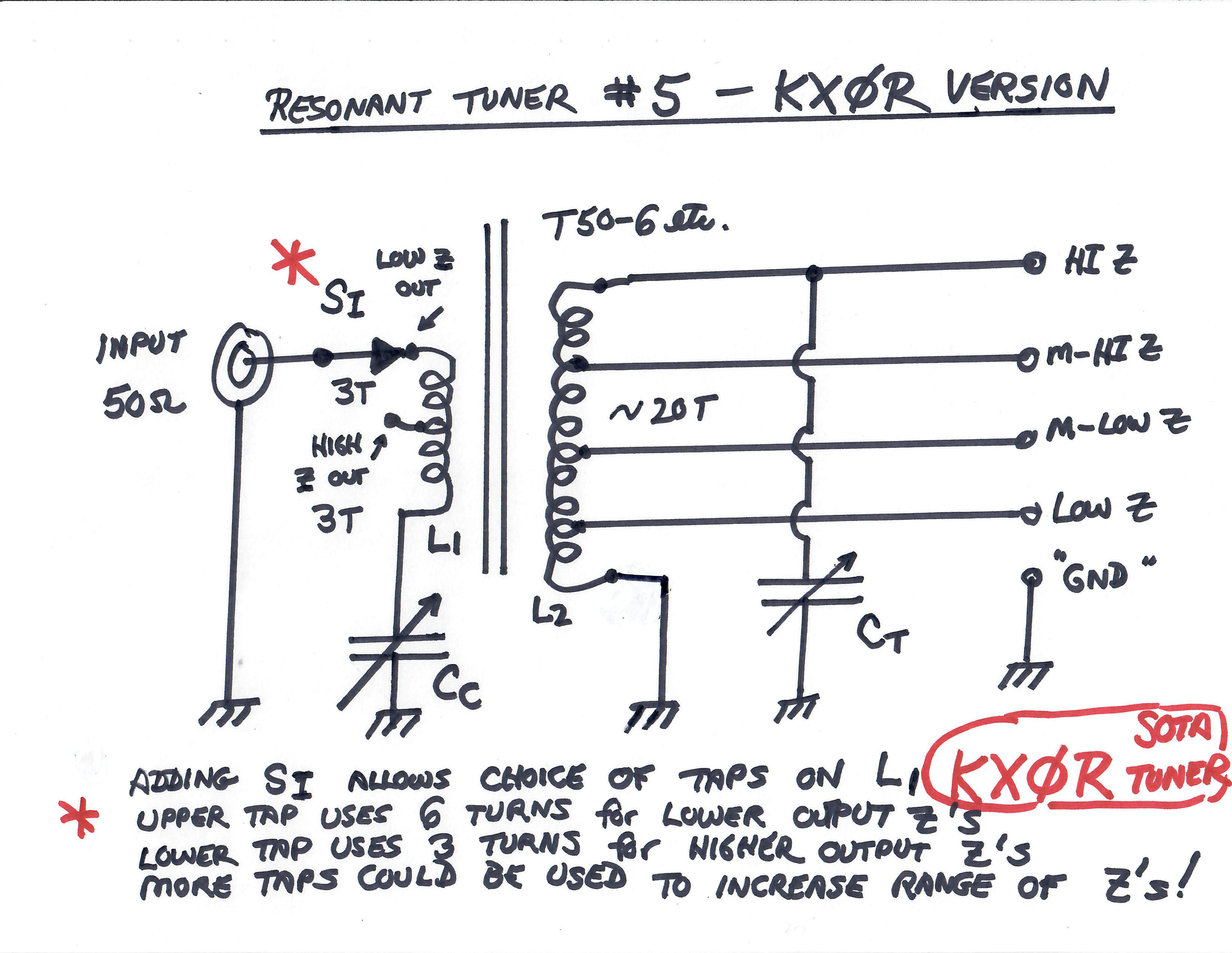
Generally, using more primary turns helps us match:

A lower frequency
A lower output impedance
Certain reactance values

Several primary taps could be included, along with a rotary switch, allowing numerous combinations of allowable impedance ranges for the total network. In practice this may be overkill, but we see this kind of control, using multiple taps on both windings, in the Fuchskreis tuners, etc.

If we try to match a single wire to operate over several amateur frequency bands, a wide range of impedances will be presented to our tuner. In practice a single primary winding is not always enough to cover all the impedance combinations we may need. Adding one switch to increase the primary is very powerful, when combined with the continuous adjustment of the variable input capacitor CC.

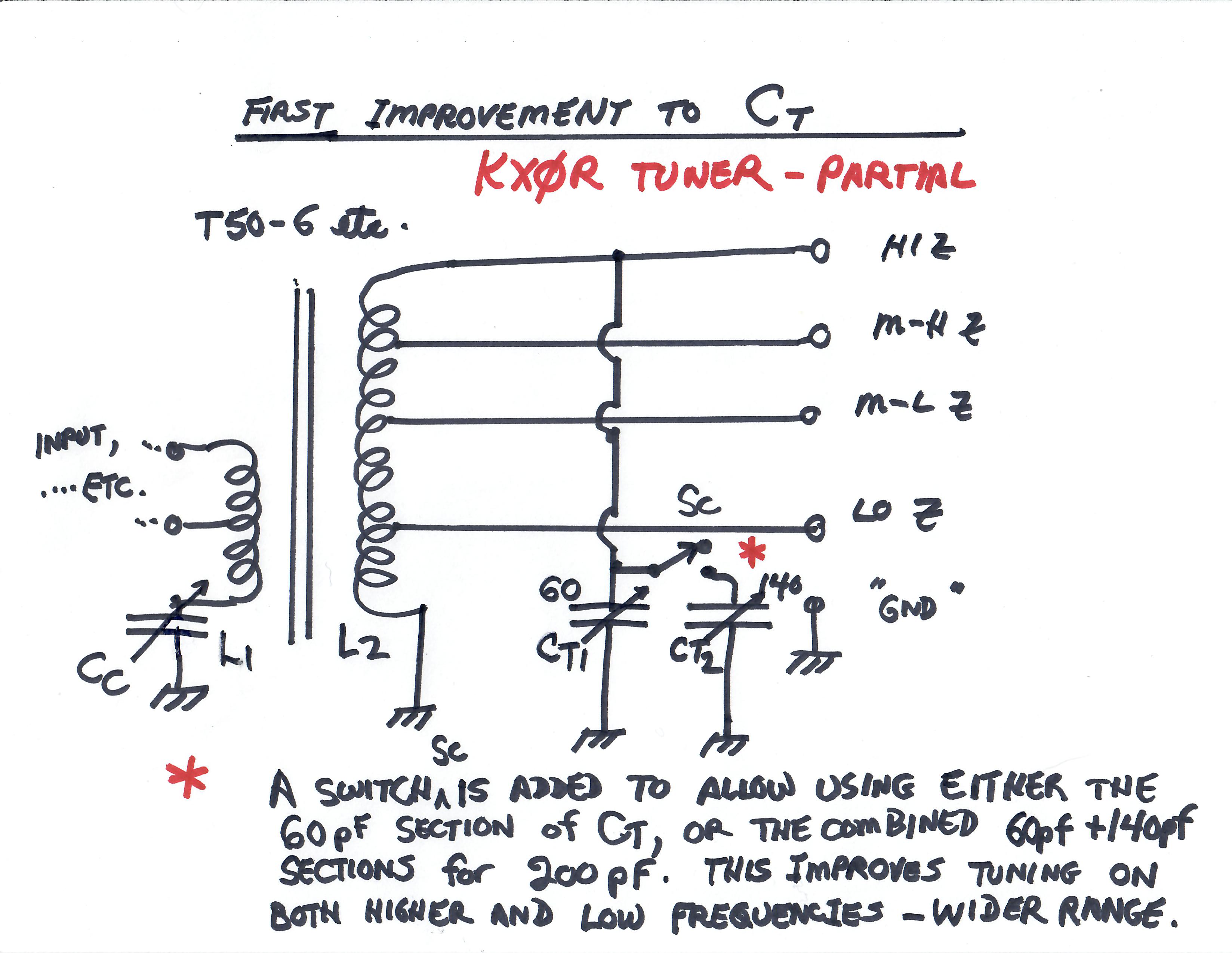
FIRST IMPROVEMENT TO CT

This is a simple change to CT. A polyvaricon capacitor with two sections is used. A small section, about 60 pF, is used for the higher frequencies. The larger section of the polyvaricon, about 140 pF, is switched in parallel by switch SC, for the lower frequencies. Using the small section has two advantages for the high frequencies:

The tuning rate is less critical – it is easier to adjust the null
The minimum capacitance is a few pF less than with both sections, extending the upper frequency limit.

The switch SC and wiring must have very low capacitance, to avoid losing the highest frequencies.

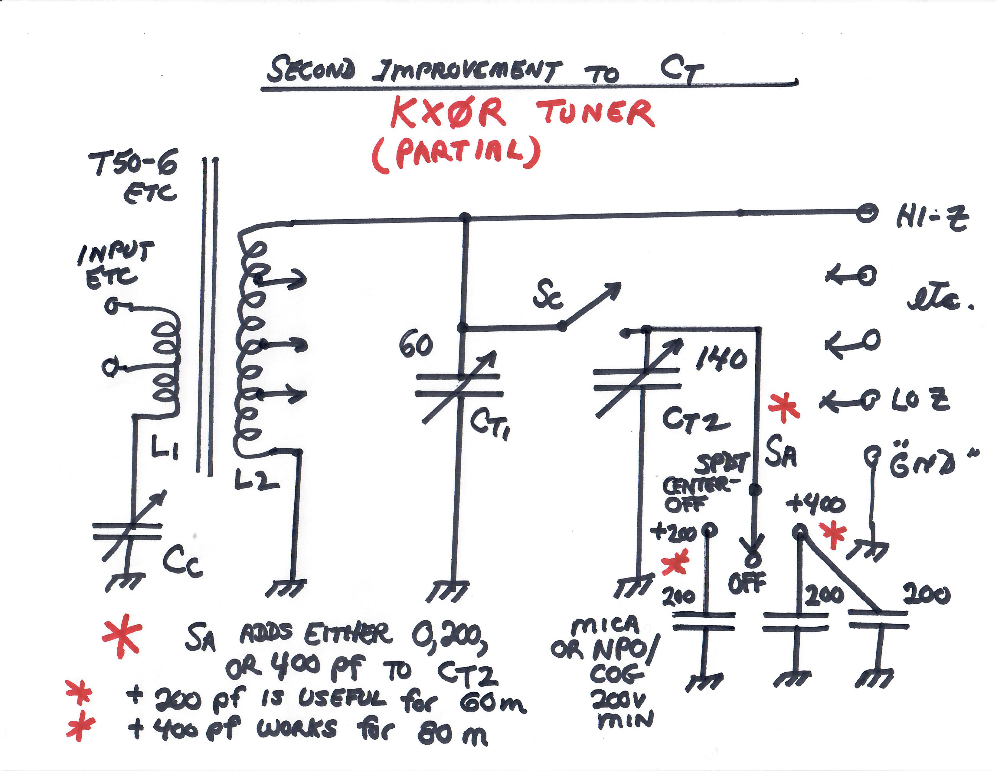
SECOND IMPROVEMENT TO CT

A switch SA is included to add fixed capacitors to the larger polyvaricon section, often ~140 pF.
A SPDT switch with a center OFF position is used for SA
Either 200 pF or 400 pF may be added.
Fixed capacitors are mica or C0G/NP0 ceramic – 200V or more.
60M and 80M bands may be tuned with the added capacitance.
Note that the new circuitry is added to the 140 pF side of the polyvaricon, so that the 60 pF section is not increased and “pulled down” by the added capacitance of SA

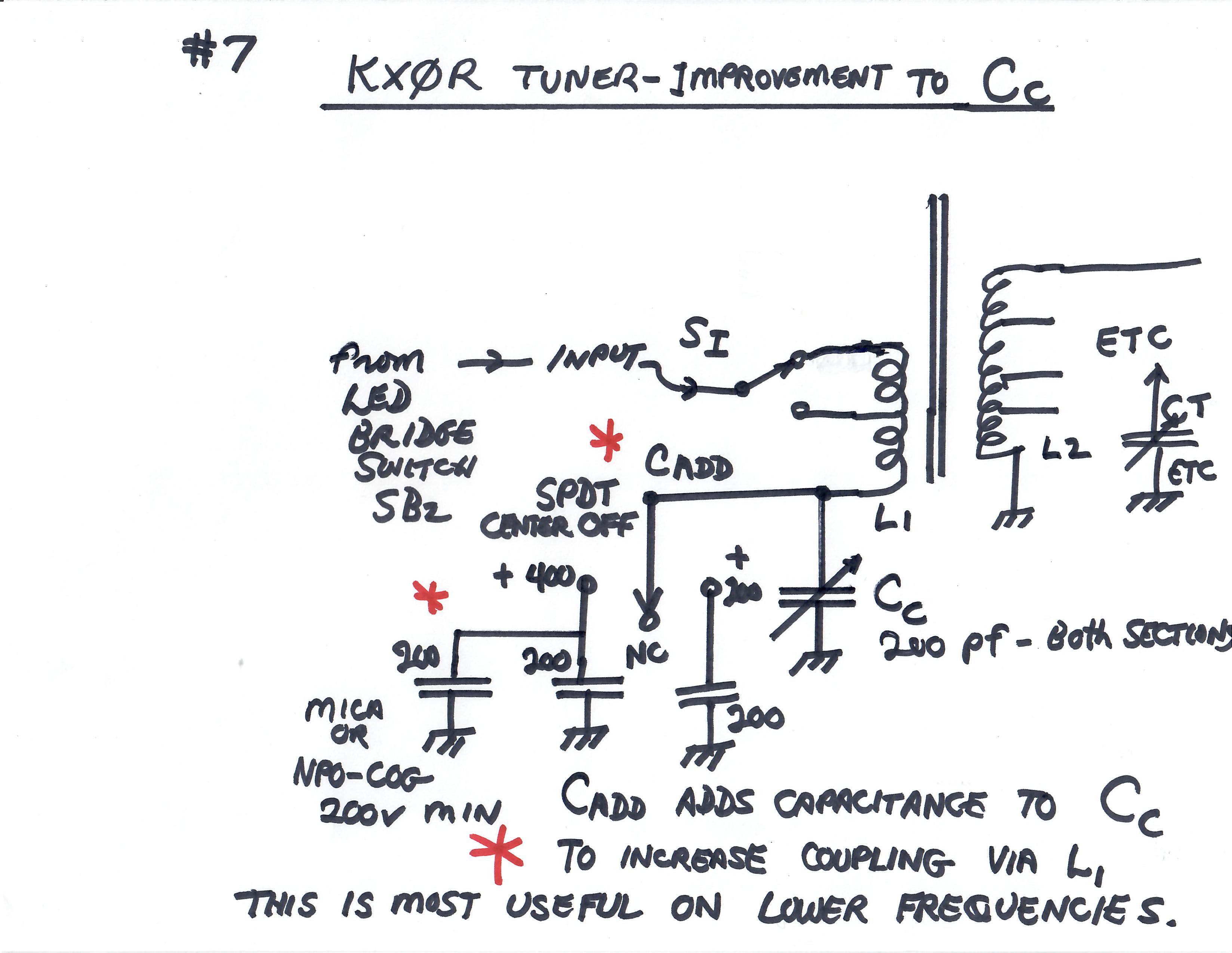
IMPROVEMENT TO CT

A switch C ADD is included to add capacitance to the input variable capacitor CC. This is a SPDT switch with center off. Either 200 or 400 pF may be added.

The added capacitance increases the coupling of L1
The adjustment range of CC is increased
Either 200 pF or 400 pF may be added.
Fixed capacitors are mica or C0G/NP0 ceramic – 200V or more.
The improvement is mostly needed on the lower frequencies

LED TUNING BRIDGE

A Dan Tayloe-type LED Bridge is included, so that the tuner may be easily adjusted. These LED bridges are included in popular tuners like the BLT, etc., and they make matching a small tuner much easier. They also provide a reasonable load for the transmitter while tuning, avoiding possible damage to the final transistors.

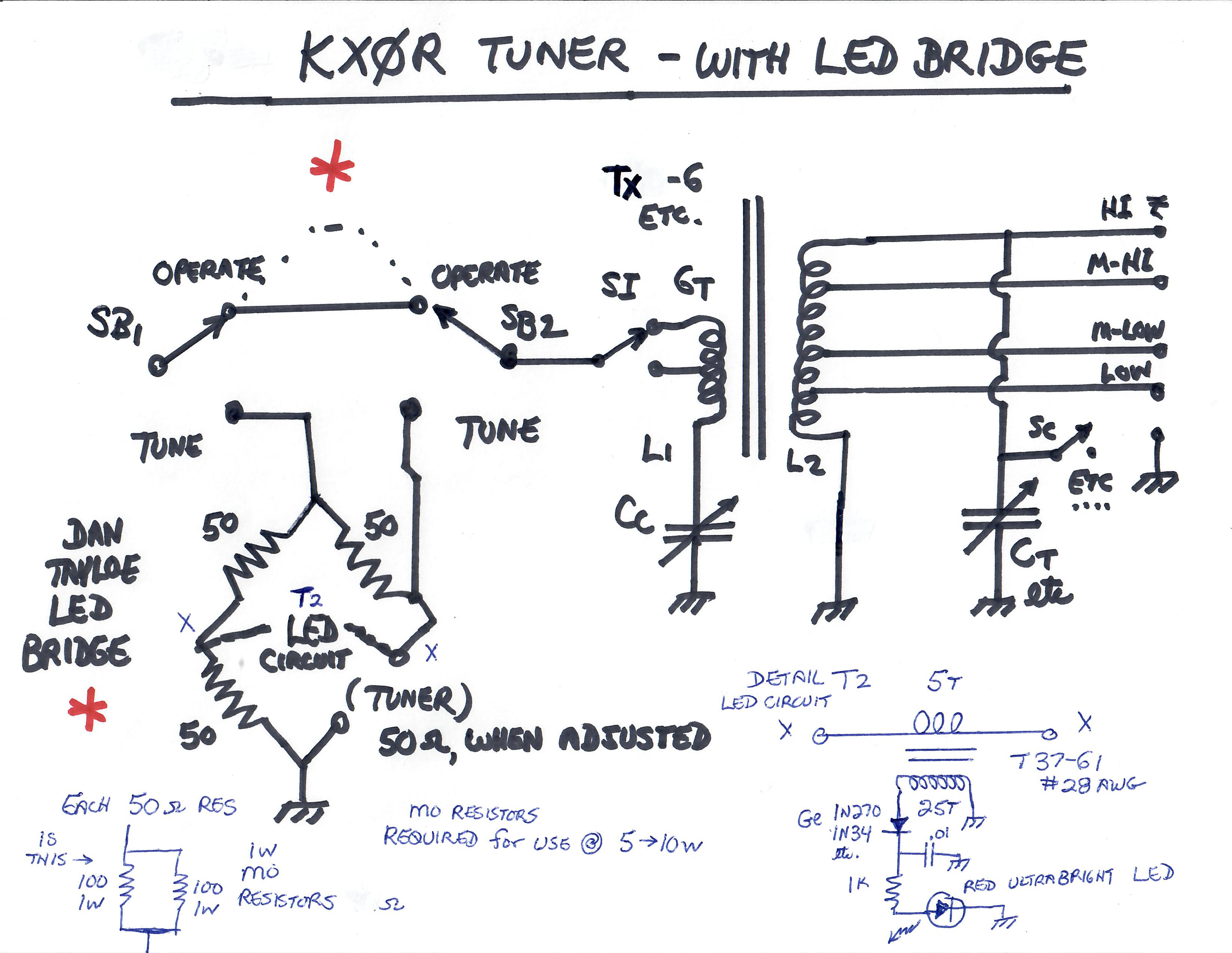
The tuning bridge is improved by using metal oxide (MO) resistors – not carbon film or carbon composition resistors. 1W and 2W MO resistors are very small, almost non-inductive, and they tolerate some abuse, not changing their value very much when overloaded slightly. If you have a 10W radio, the bridge resistors should be able to withstanding the full 10W for a few seconds without damage. I use a parallel pair of 100 ohm MO resistors for each 50 ohm bridge resistor. Use the best you can find – some small ones are rated for 2W.

Tuning should be done at low power, usually around 1-2W input, to avoid stressing the bridge resistors. If you forget and start calling CQ with the bridge switch in the TUNE position, so you have ¾ of your 10W going into the bridge resistors – this is 2.5W for each 50-ohm arm, or 1.25W per 100-ohm resistor, if they’re in parallel pairs. You may make several contacts before you discover the error – I have! That’s when you need the better MO resistors!

Choose a non-diffused, ultra-bright or ultra-super-bright LED, rated at 2000 mcd or more. These are worth their cost, and they will make your SOTA life better! The LED should be painfully bright if viewed indoors. You must be able to null the bridge outdoors, even in full sun.

If the bridge is built small and symmetric, it will look like 50 ohms when the tuner is matched, because the tuner itself will be one of the four 50-ohm legs of the bridge. The null of the LED also should occur when all four legs are 50 ohms. Unfortunately errors may exist in these bridges, depending on how they are built, due to stray capacitance and inductance.

I was able to improve the accuracy of my bridges by adding small compensating capacitances, usually in the range of 10-30 pF, across one or more of the bridge resistors. Using a well-calibrated MFJ-259B analyzer, and an accurate 50 ohm load, I was able to improve the accuracy of my nulls above 14 MHz. Compensation is a fine point, not really necessary, but it’s nice to know that when the LED is out, the impedance of the tuner, as well as the bridge, is very close to 50 ohms.

When the LED bridge is bypassed, Operate Mode, a little RF leaks across the switch, and the LED lights slightly when the radio is keyed. This little defect is useful for seeing that the RF is going out.

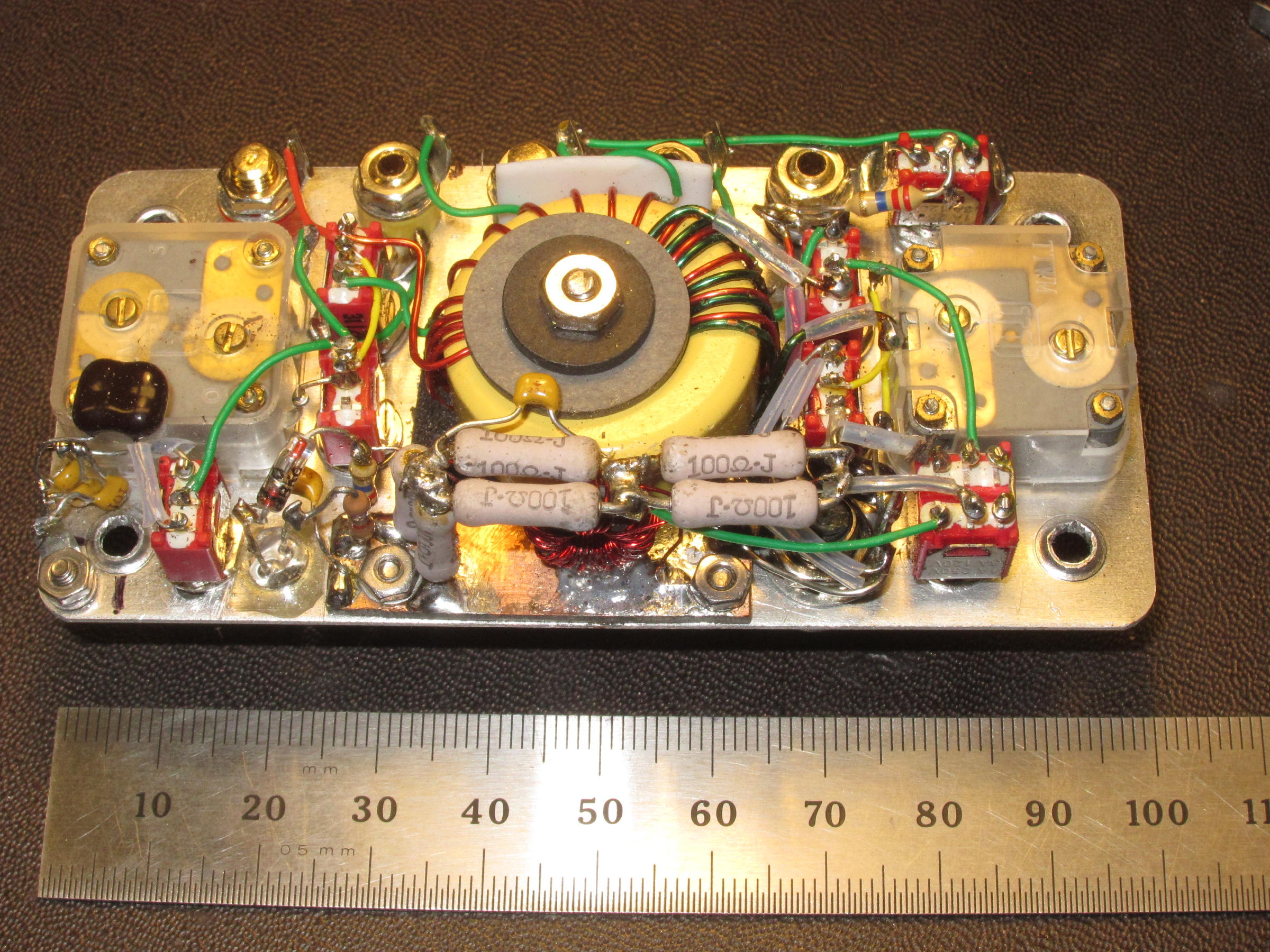
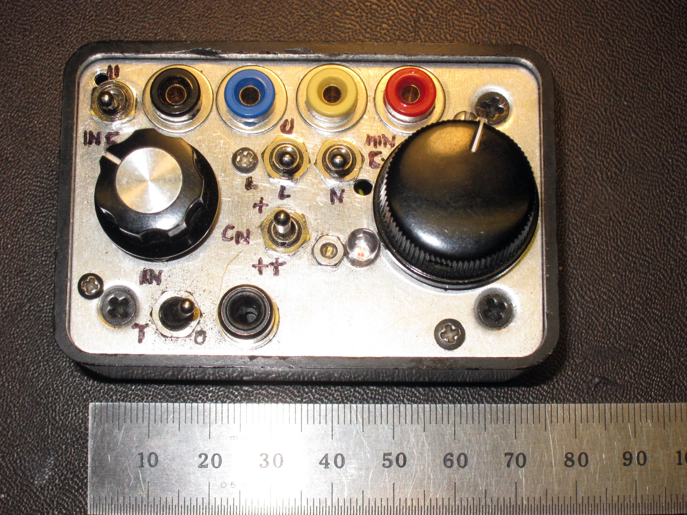
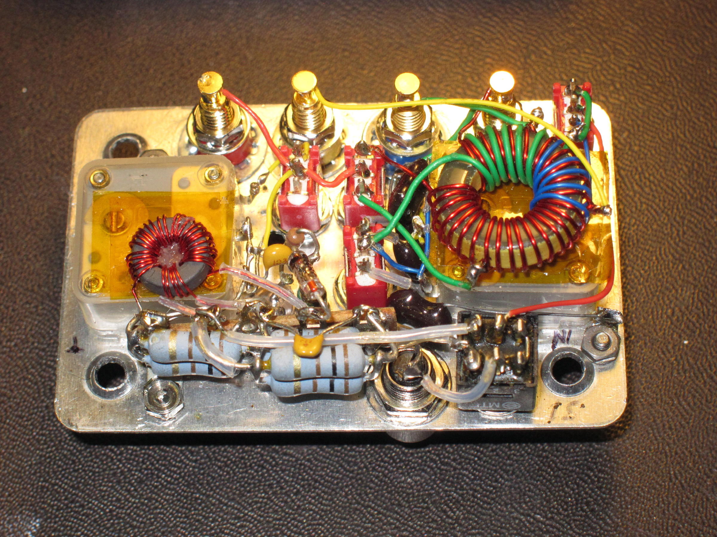
ACTUAL KX0R CIRCUITS

Here are two KX0R tuners. One is larger than the other. Hopefully these will be useful to build a tuner using the ideas presented here. This is not a how-to-make-it article – experience and improvisation are required.