Part I: Calculating the Magnetization Admittance of a Ferrite Toroidal Winding
Introduction
If one is to understand something about ferrite and how it behaves, some understanding of the magnetization admittance is required. The magnetization admittance will provide a means to estimate the power dissipations of ferrite transformers and inductors, their efficiencies, and their power handling capabilities. A little bit of messy algebra is required for understanding, but it’s worth it. Ferrite is ubiquitous. It’s in many of our rigs, antenna tuners, filters, baluns, and power supplies.
Historical Information
Let’s begin with a bit of historical information about an antenna and its antenna matching device that has recently assumed the form of a ferrite transformer. This history is a bit narrow, but I hope that you will see what I am driving at later on.
Ferrite transformer-fed End-Fed Half-Wave (EFHW) antennas have grown in popularity in recent years due to their ability to operate on multiple bands in reduced spaces. Some of these antennas have been optimized for use on multiple bands by placing a small compensating inductor near the location of the first current maximum for the highest band of operation.
There is a hint to the origin of the multiband EFHW antenna on the MyAntennas website [1]. Danny Horvat, N4EXA (a.k.a. E73M), provides an interesting reference to some writing about the antenna in Karl Rothammel’s (Y21BK) Antennen Buch [2]. The cover, Figure 1, of the 12th edition shows a drawing of harmonics on a wire antenna. The drawing shows an inductor located at the position of the first current peak of the highest order harmonic on the wire. Rothammel’s book attributes the design to Gerhard Bäz, DL7AB. Frank Dorenberg [3], N4SPP, was kind enough to forward a copy of the original journal article for this antenna that appeared in an October 1949 issue of the radio journal Funk-Technik [4] on pages 576 and 577. The compensating inductor has little effect on fundamental operation, but it has an enormous effect when the antenna is used for harmonic operation. The inductance and placement of this inductor have been analyzed in EZNEC and will be the subject of a future article. Danny, E73M, also makes reference to a transformer [5] invented by Nikola Tesla in 1897. A version of Tesla’s transformer appears in the antenna patent [6] of Joseph Fuchs, OE1JF, in 1928.
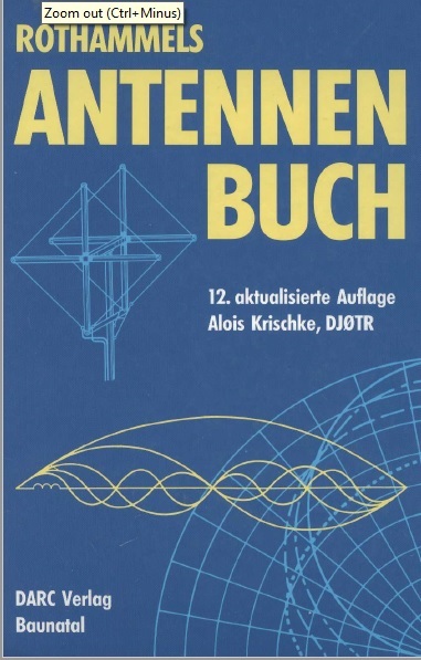
Figure 1. Cover of Rothammel’s Antennen Buch, 12th ed. An antenna wire in harmonic operation is shown. A little inductor is located at the first current maximum for the 10m band.
Recently, the ARRL has offered a popular, inexpensive do-it-yourself kit to make an EFHW antenna [7]. Similar, ready-made versions are available from multiple sources such as MyAntennas [8], MFJ [9], PAR/LNR Precision [10], and HyEndFed [11], to name just a few. Some use the compensating inductor, while some do not. The ARRL transformer will be the subject of a worked example in Part II of this article. The ARRL antenna wire does not make use of the compensating inductor, but it may be added.
In spite of their omnipresence and popularity, there has been very little published on the subject of how the ferrite transformer version of the end-fed antenna feed actually works and how much power it can handle.
After searching the literature and the web, I came upon the blog of Owen Duffy, VK1OD. His website [12] is rich with content on the subject of ferrite. Not unlike any good teacher, he is fond of leaving calculations as a challenge to the reader. A good place to begin is with the magnetization admittance.
The Interwinding Capacitance and Magnetization Admittance
Magnetization admittances for the windings on ferrite cores are required to calculate losses in ferrite cores used in inductor and transformer applications. Owen Duffy has provided an excellent paper [13] on the subject that is somewhat short in detail. This article attempts to provide the missing steps in order to make his paper on the subject of ferrite more accessible.
In his paper, the complex impedance of a 10-turn winding on an FT140-43 ferrite core at 21 MHz has been provided as the starting point. This value could have been measured with an antenna analyzer, with a network analyzer, or could have been calculated from the manufacturer’s complex permeability data. We demonstrate how the complex impedance is derived from the complex permeability data in a separate paper.
The value of the interwinding capacitance should be included in the impedance calculation to compute the magnetization admittance value with greater accuracy. Not only is there an interwinding capacitance, but there is also capacitive coupling between primary and secondary windings. The interwinding capacitance is modeled in parallel with the winding impedance. D.W. Knight [14] has measured interwinding capacitance values for several windings on ferrite cores. The value of interwinding capacitance will have a large effect on the magnetization admittance.
If the interwinding capacitance is 2 pf at the design frequency of 21 MHz, the capacitive reactance calculated from,

will be,
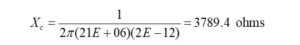
The interwinding capacitive reactance that is in parallel with the winding impedance is 3789.4 ohms.
Digression:
The subject of complex numbers is something that we seldom see in use in everyday life. If this all seems new to you, please follow along. The expressions can be messy, but they all work out. These days, circuit modeling replaces these messy calculations, but it’s good to perform them by hand at least once for understanding.
The complex impedance is composed of two parts, a purely resistive part called the real part and a purely reactive part called the imaginary part. The letter i or j in front of the reactive part lets us know that it is the imaginary part. The other thing that we must remember is that i or j is defined by,

and

If we multiply i or j by itself, we get -1. We will make use of this property when we begin to multiply complex numbers together.
Regression:
Suppose that the winding impedance on our ferrite core has been determined to be 2627 + j 2044 by derivation from the manufacturer’s data. There are two methods to calculate the parallel combination of the interwinding capacitive reactance with the winding impedance. The first method makes use of the formula

for which,
Z1 = 2627 + j2044
where +j denotes an inductive reactance. Since there is a real part, the phase angle is other than +90°.
Z2 = 0 – j3789.4
Since there is no real part, the -j denotes a capacitive reactance whose voltage lags the current by 90°.
Method I
Entering the values into the equation, we obtain

we could multiply out all of the terms in the numerator and combine the terms and rationalize the denominator, or we could convert the expressions to polar form.
In order to accomplish this, we must first find the magnitude of Z1,
![]()
where RE is the real part of Z1 and IM is the imaginary part of Z1.

Next, we must find the phase angle,


In polar form

Similarly, for Z2, because there is no real part, the magnitude is just

A few more words about the phase angle in AC circuits for pure resistors, capacitors, and inductors – in a resistor, the voltage and current are in phase, so

In a capacitor, the voltage lags the current by 90° because it requires time for the capacitor to charge up, so

In an inductor, the voltage leads the current by 90° because the inductor opposes the flow of current, so

Thus, the phase angle for the parallel capacitor,

If the impedance possesses both real and imaginary parts, there will be a phase angle other than ±90°.
In polar form for the interwinding capacitance,
![]()
Next, we need to combine terms in the denominator before converting to polar form,
![]()
The magnitude of the denominator is given by,
![]()
The phase angle of the denominator is given by,

The denominator may be written in polar form,
![]()
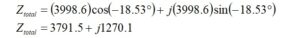
Finally, the expression for Ztotal may be written in polar form,
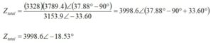
This may be converted back to rectangular form with some help from the Euler identity,

where,
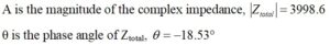
Substituting
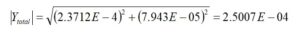
The easiest way to obtain the magnetization admittance is to work with the polar form of Ztotal
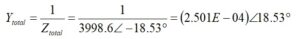
In order to calculate the core loss, it is necessary to obtain the real part of the magnetization admittance, the conductance, by conversion back to rectangular form,
The real part of Ytotal is the conductance, G, in units of Siemens,
G = 2.371E-04 Siemens
The imaginary part of Ytotal is the susceptance, B, in units of Siemens
B = 7.948E-5 Siemens
Method II
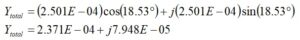
There is a second method for obtaining the magnetization admittance. This may be calculated by adding the individual admittances of the winding and the interwinding capacitance.

We won’t be able to add the admittances in polar form unless the phase angles are the same, in which case the phasors lie on the same line. We must first convert to rectangular form and then convert back to polar form.

The second term may be written by inspection, but it is best not to leave out any steps. That means that the denominators have to be rationalized first to free them of imaginary numbers. If you have forgotten how to do this, the method is shown below. You multiply the top and bottom of each factor by the complex conjugate of their respective denominators. To obtain the complex conjugate, you just invert the sign of the imaginary part.
which is rectangular form. This form provides the real part of the admittance, which is the conductance value, G, required to calculate the ferrite loss,
G = 2.371E-04 Siemens
as before.
In order to convert to polar form, the procedure in the first method is repeated. The magnitude of the admittance is given by,
The phase angle is given by,

The polar form may be written
![]()
Power Lost to the Ferrite Core
Now that the value of the conductance, G, has been obtained using both methods, it is possible to calculate the percentage of power lost to the ferrite core,
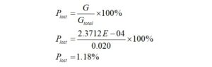
where
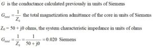
For this 10-turn inductor on FT140-43 at 21 MHz, the power lost to the core expressed as a percent is 1.18%.
The subject of heat dissipation in ferrite transformers and inductors is treated in Part II of this article.
References
[1] https://myantennas.com/wp/efhw-8010-is-this-the-ultimate-magic-antenna/
[2] Rothammel, Karl, Antennen Buch, 12th ed., Deutscher Amateur Radio Club (DARC), pp. 228-229.
[3] https://www.nonstopsystems.com/radio/frank_radio_antenna_multiband_end-fed.htm
[4] https://nvhrbiblio.nl/biblio/tijdschrift/Funktechnik/1949/FT_1949_Heft_19-OCR.pdf
[5] https://teslauniverse.com/nikola-tesla/patents/us-patent-593138-electrical-transformer
[6] http://www.antentop.org/016/files/oe1jf_016.pdf
[7] https://home.arrl.org/action/Store/Product-Details/productId/133267
[8] MyAntennas, op. cit.
[9] https://mfjenterprises.com/collections/all/products/mfj-1982hp
[10] https://www.parelectronics.com/end-fedz.php
[11] https://www.hyendcompany.nl/antenna/multiband_8040302017151210m#main
[12] https://owenduffy.net/blog/
[13] https://owenduffy.net/files/EstimateZFerriteToroidInductor.pdf
[14] https://www.g3ynh.info/zdocs/magnetics/appendix/self_res/self-res.pdf
No comments:
Post a Comment